Data Science Portfolio

House Prices: Advanced Regression Techniques

Introduction

This project is for the Kaggle competition House Prices: Advanced Regression Techniques. The dataset can be found on the competition page here:

https://www.kaggle.com/c/house-prices-advanced-regression-techniques/overview

The data consists of 81 total variables, many of which are redundant and/or unnecessary. Our target variable which we are trying to predict is SalePrice.

We will first examine our features through visualizations, and then do feature engineering. Finally, we will do three iterations of model building:

1) Simple feature selection based on manual inspection

2) Feature importances from random forest regression

3) Principal Components Analysis

Preparing the Data

Loading the Data

import sys
import time
import numpy as np
import pandas as pd
import scipy
import matplotlib.pyplot as plt
import seaborn as sns
from sklearn.svm import SVC
from sklearn import ensemble
from sklearn import linear_model
from sklearn import neighbors
from sklearn.linear_model import LinearRegression
from sklearn.linear_model import Ridge
from sklearn.linear_model import Lasso
from sklearn.ensemble import RandomForestRegressor
from sklearn.ensemble import RandomForestClassifier
from sklearn.model_selection import cross_val_score
from sklearn.feature_selection import SelectKBest, f_classif
from matplotlib.mlab import PCA as mlabPCA
from sklearn.preprocessing import StandardScaler
from sklearn.preprocessing import LabelEncoder
from sklearn.decomposition import PCA
from sklearn.model_selection import train_test_split
from sklearn.metrics import precision_recall_curve
from sklearn.metrics import average_precision_score
from sklearn.metrics import classification_report
from sklearn.metrics import mean_squared_error
from sklearn.impute import SimpleImputer
from sklearn.model_selection import GridSearchCV
from sklearn.pipeline import Pipeline
import statsmodels.formula.api as smf
from scipy import stats
from scipy.stats import normaltest
from scipy.special import boxcox1p
from scipy.stats import norm
from scipy.stats import skew
%matplotlib inline
np.set_printoptions(threshold=sys.maxsize)
pd.set_option("display.max_rows", 100)

df_train = pd.read_csv('train.csv')
df_train.head()

	Id	MSSubClass	MSZoning	LotFrontage	LotArea	Street	Alley	LotShape	LandContour	Utilities	...	PoolArea	PoolQC	Fence	MiscFeature	MiscVal	MoSold	YrSold	SaleType	SaleCondition	SalePrice
0	1	60	RL	65.0	8450	Pave	NaN	Reg	Lvl	AllPub	...	0	NaN	NaN	NaN	0	2	2008	WD	Normal	208500
1	2	20	RL	80.0	9600	Pave	NaN	Reg	Lvl	AllPub	...	0	NaN	NaN	NaN	0	5	2007	WD	Normal	181500
2	3	60	RL	68.0	11250	Pave	NaN	IR1	Lvl	AllPub	...	0	NaN	NaN	NaN	0	9	2008	WD	Normal	223500
3	4	70	RL	60.0	9550	Pave	NaN	IR1	Lvl	AllPub	...	0	NaN	NaN	NaN	0	2	2006	WD	Abnorml	140000
4	5	60	RL	84.0	14260	Pave	NaN	IR1	Lvl	AllPub	...	0	NaN	NaN	NaN	0	12	2008	WD	Normal	250000

5 rows × 81 columns

df_train.describe()

	Id	MSSubClass	LotFrontage	LotArea	OverallQual	OverallCond	YearBuilt	YearRemodAdd	MasVnrArea	BsmtFinSF1	...	WoodDeckSF	OpenPorchSF	EnclosedPorch	3SsnPorch	ScreenPorch	PoolArea	MiscVal	MoSold	YrSold	SalePrice
count	1460.000000	1460.000000	1201.000000	1460.000000	1460.000000	1460.000000	1460.000000	1460.000000	1452.000000	1460.000000	...	1460.000000	1460.000000	1460.000000	1460.000000	1460.000000	1460.000000	1460.000000	1460.000000	1460.000000	1460.000000
mean	730.500000	56.897260	70.049958	10516.828082	6.099315	5.575342	1971.267808	1984.865753	103.685262	443.639726	...	94.244521	46.660274	21.954110	3.409589	15.060959	2.758904	43.489041	6.321918	2007.815753	180921.195890
std	421.610009	42.300571	24.284752	9981.264932	1.382997	1.112799	30.202904	20.645407	181.066207	456.098091	...	125.338794	66.256028	61.119149	29.317331	55.757415	40.177307	496.123024	2.703626	1.328095	79442.502883
min	1.000000	20.000000	21.000000	1300.000000	1.000000	1.000000	1872.000000	1950.000000	0.000000	0.000000	...	0.000000	0.000000	0.000000	0.000000	0.000000	0.000000	0.000000	1.000000	2006.000000	34900.000000
25%	365.750000	20.000000	59.000000	7553.500000	5.000000	5.000000	1954.000000	1967.000000	0.000000	0.000000	...	0.000000	0.000000	0.000000	0.000000	0.000000	0.000000	0.000000	5.000000	2007.000000	129975.000000
50%	730.500000	50.000000	69.000000	9478.500000	6.000000	5.000000	1973.000000	1994.000000	0.000000	383.500000	...	0.000000	25.000000	0.000000	0.000000	0.000000	0.000000	0.000000	6.000000	2008.000000	163000.000000
75%	1095.250000	70.000000	80.000000	11601.500000	7.000000	6.000000	2000.000000	2004.000000	166.000000	712.250000	...	168.000000	68.000000	0.000000	0.000000	0.000000	0.000000	0.000000	8.000000	2009.000000	214000.000000
max	1460.000000	190.000000	313.000000	215245.000000	10.000000	9.000000	2010.000000	2010.000000	1600.000000	5644.000000	...	857.000000	547.000000	552.000000	508.000000	480.000000	738.000000	15500.000000	12.000000	2010.000000	755000.000000

8 rows × 38 columns

df_train.shape

(1460, 81)

Before we start, let’s drop Id since it is unnecessary for our analysis.

df_train.drop('Id', axis=1, inplace=True)
df_train.describe()

	MSSubClass	LotFrontage	LotArea	OverallQual	OverallCond	YearBuilt	YearRemodAdd	MasVnrArea	BsmtFinSF1	BsmtFinSF2	...	WoodDeckSF	OpenPorchSF	EnclosedPorch	3SsnPorch	ScreenPorch	PoolArea	MiscVal	MoSold	YrSold	SalePrice
count	1460.000000	1201.000000	1460.000000	1460.000000	1460.000000	1460.000000	1460.000000	1452.000000	1460.000000	1460.000000	...	1460.000000	1460.000000	1460.000000	1460.000000	1460.000000	1460.000000	1460.000000	1460.000000	1460.000000	1460.000000
mean	56.897260	70.049958	10516.828082	6.099315	5.575342	1971.267808	1984.865753	103.685262	443.639726	46.549315	...	94.244521	46.660274	21.954110	3.409589	15.060959	2.758904	43.489041	6.321918	2007.815753	180921.195890
std	42.300571	24.284752	9981.264932	1.382997	1.112799	30.202904	20.645407	181.066207	456.098091	161.319273	...	125.338794	66.256028	61.119149	29.317331	55.757415	40.177307	496.123024	2.703626	1.328095	79442.502883
min	20.000000	21.000000	1300.000000	1.000000	1.000000	1872.000000	1950.000000	0.000000	0.000000	0.000000	...	0.000000	0.000000	0.000000	0.000000	0.000000	0.000000	0.000000	1.000000	2006.000000	34900.000000
25%	20.000000	59.000000	7553.500000	5.000000	5.000000	1954.000000	1967.000000	0.000000	0.000000	0.000000	...	0.000000	0.000000	0.000000	0.000000	0.000000	0.000000	0.000000	5.000000	2007.000000	129975.000000
50%	50.000000	69.000000	9478.500000	6.000000	5.000000	1973.000000	1994.000000	0.000000	383.500000	0.000000	...	0.000000	25.000000	0.000000	0.000000	0.000000	0.000000	0.000000	6.000000	2008.000000	163000.000000
75%	70.000000	80.000000	11601.500000	7.000000	6.000000	2000.000000	2004.000000	166.000000	712.250000	0.000000	...	168.000000	68.000000	0.000000	0.000000	0.000000	0.000000	0.000000	8.000000	2009.000000	214000.000000
max	190.000000	313.000000	215245.000000	10.000000	9.000000	2010.000000	2010.000000	1600.000000	5644.000000	1474.000000	...	857.000000	547.000000	552.000000	508.000000	480.000000	738.000000	15500.000000	12.000000	2010.000000	755000.000000

8 rows × 37 columns

Dropping Outliers

The dataset documentation indicates that there are five outliers that should be removed prior to proceeding with the data (four in the training set). These outliers can be easily seen from the scatter plot of SalePrice vs. GrLivArea. Let’s write a simple function that allows us to easily plot a single scatter plot.

# Function to easily plot a single scatter plot
def scatter_plot_single(df, target, col):
    plt.scatter(x=df[col], y=df[target])
    plt.xlabel(col)
    plt.ylabel(target)
    plt.title(target + ' vs. ' + col)

scatter_plot_single(df_train, 'SalePrice', 'GrLivArea')

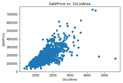
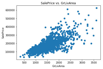
We can see the four outliers in question. Two of them are very low-priced houses with a high GrLivArea. The other three simply appear to be expensive houses that are still following the trend. The documentation recommends us to get rid of these outliers before processing the data further, so let’s do that.

# Check shape
df_train.shape

(1460, 80)

df_train = df_train.drop(df_train[(df_train['GrLivArea']>4000)].index)

# Check shape again
df_train.shape

(1456, 80)

# Plot again for visual check
scatter_plot_single(df_train, 'SalePrice', 'GrLivArea')

# Check shape
df_train.shape

(1456, 80)

Exploring the Data

Univariate Data

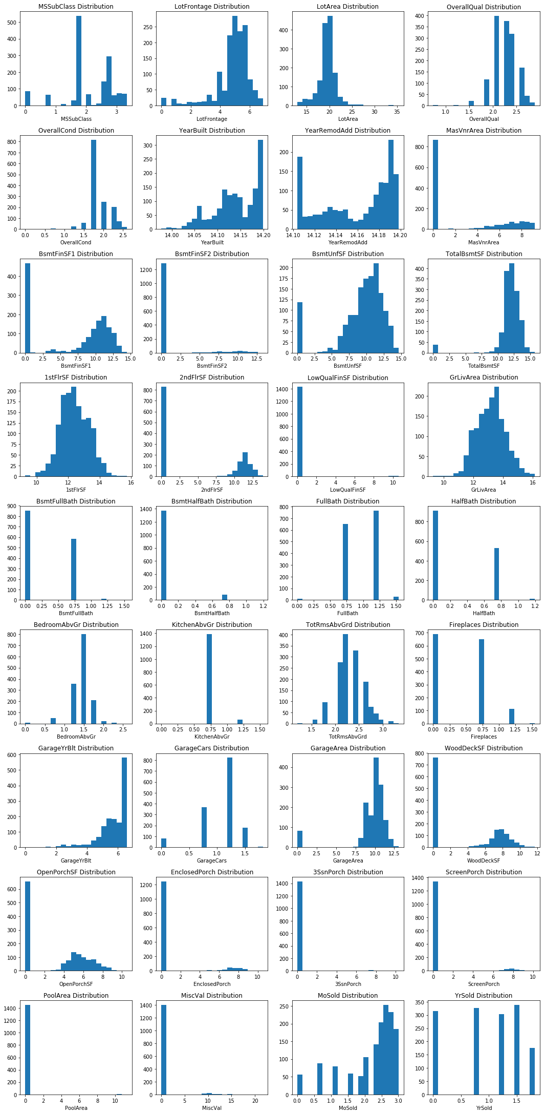
Let’s plot the distributions for each of our continuous features. We can write a function to do this.

cols = ['MSSubClass', 'LotFrontage', 'LotArea', 'OverallQual', 'OverallCond', 
        'YearBuilt', 'YearRemodAdd', 'MasVnrArea', 'BsmtFinSF1', 'BsmtFinSF2', 
        'BsmtUnfSF', 'TotalBsmtSF', '1stFlrSF', '2ndFlrSF', 'LowQualFinSF', 
        'GrLivArea', 'BsmtFullBath', 'BsmtHalfBath', 'FullBath', 'HalfBath',
        'BedroomAbvGr', 'KitchenAbvGr', 'TotRmsAbvGrd', 'Fireplaces', 'GarageYrBlt', 
        'GarageCars', 'GarageArea', 'WoodDeckSF', 'OpenPorchSF', 'EnclosedPorch', 
        '3SsnPorch', 'ScreenPorch', 'PoolArea', 'MiscVal', 'MoSold', 'YrSold']

# Function to neatly plot multiple histograms
def histogram_multiple(df, cols, figsize_x, figsize_y, nrows, ncols):
    i = 1
    plt.figure(figsize=(figsize_x, figsize_y))
    
    for col in cols:
        plt.subplot(nrows,ncols,i)
        plt.hist(df[col], bins=20)
        plt.xlabel(col)
        plt.title(col + ' Distribution')
        i += 1
    
    plt.tight_layout()
    plt.show()

histogram_multiple(df_train, cols, 15, 50, 15, 4)

Feature-Target Relationships

Continuous Features

Now let’s visualize the relationship between SalePrice and all of our continuous features. We can write a function to easily create a scatter plot for any given x and y with our desired parameters. First let’s put all the column names for our continuous variables into a list.

# Function to easily plot a single scatter plot
def scatter_plot_single(df, target, col):
    plt.scatter(x=df[col], y=df[target])
    plt.xlabel(col)
    plt.ylabel(target)
    plt.title(target + ' vs. ' + col)
     
# Function to neatly plot multiple scatter plots
def scatter_plot_multiple(df, target, cols, figsize_x, figsize_y, nrows, ncols):
    i = 1
    plt.figure(figsize=(figsize_x, figsize_y))
    
    for col in cols:
        if col != target:
            plt.subplot(nrows,ncols,i)
            scatter_plot_single(df, target, col)
            i += 1
    
    plt.tight_layout()
    plt.show()

Now we can use this to neatly visualize scatter plots of SalePrice with many different input features all in one place. For the amount of features we have, we can use nine rows and four columns.

df_train.head()

	MSSubClass	MSZoning	LotFrontage	LotArea	Street	Alley	LotShape	LandContour	Utilities	LotConfig	...	PoolArea	PoolQC	Fence	MiscFeature	MiscVal	MoSold	YrSold	SaleType	SaleCondition	SalePrice
0	60	RL	65.0	8450	Pave	NaN	Reg	Lvl	AllPub	Inside	...	0	NaN	NaN	NaN	0	2	2008	WD	Normal	208500
1	20	RL	80.0	9600	Pave	NaN	Reg	Lvl	AllPub	FR2	...	0	NaN	NaN	NaN	0	5	2007	WD	Normal	181500
2	60	RL	68.0	11250	Pave	NaN	IR1	Lvl	AllPub	Inside	...	0	NaN	NaN	NaN	0	9	2008	WD	Normal	223500
3	70	RL	60.0	9550	Pave	NaN	IR1	Lvl	AllPub	Corner	...	0	NaN	NaN	NaN	0	2	2006	WD	Abnorml	140000
4	60	RL	84.0	14260	Pave	NaN	IR1	Lvl	AllPub	FR2	...	0	NaN	NaN	NaN	0	12	2008	WD	Normal	250000

5 rows × 80 columns

continuous_feature_names = df_train.select_dtypes(['float64','int64']).columns
scatter_plot_multiple(df_train, 'SalePrice', continuous_feature_names, 15, 50, 15, 4)

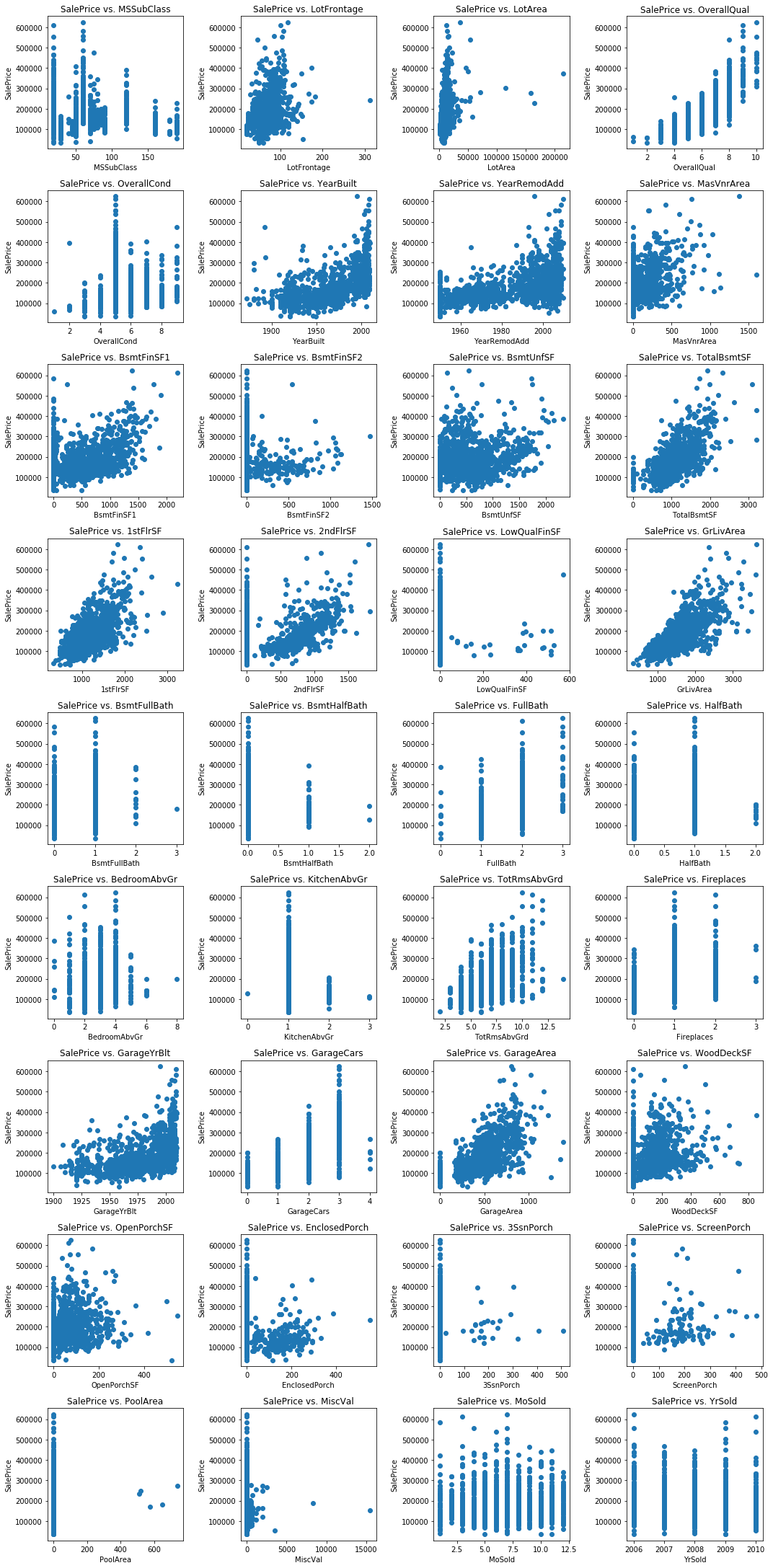
The following features exhibit a strong linear relationship with SalePrice:

• LotFrontage
• TotalBsmtSF
• 1stFlrSF
• GrLivArea
• GarageArea

The following features exhibit a weak linear relationship with SalePrice:

• LotArea
• MasVnrArea
• BsmtFinSF1
• BsmtUnfSF
• WoodDeckSF
• OpenPorchSF
• PoolArea

We will transform the nonlinear features in order to linearize them prior to modeling.

Categorical Features

Now let’s visualize some categorical variables to see how they relate to SalePrice. First let’s plot a boxplot of SalePrice vs. OverallQual.

var = 'OverallQual'
data = pd.concat([df_train['SalePrice'], df_train[var]], axis=1)
f, ax = plt.subplots(figsize=(8, 6))
fig = sns.boxplot(x=var, y="SalePrice", data=data)
fig.axis(ymin=0, ymax=800000);

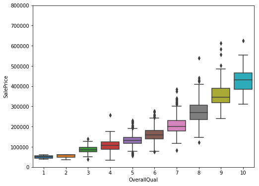
We can clearly see that as the owner-reported overall quality rating increases, the SalePrice increases as well, which makes sense. We would expect higher-priced homes to be of better quality. Now let’s take a look at SalePrice vs. YearBuilt.

var = 'YearBuilt'
data = pd.concat([df_train['SalePrice'], df_train[var]], axis=1)
f, ax = plt.subplots(figsize=(16, 8))
fig = sns.boxplot(x=var, y="SalePrice", data=data)
fig.axis(ymin=0, ymax=800000);
plt.xticks(rotation=90);

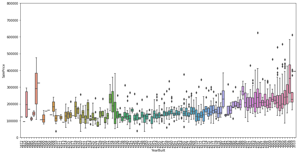
The home selling price does appear to increase slightly over time, aside from some odd outliers at the far left end of the scale (late 1800s).

Our target variable is SalePrice, so our objective will be to predict a home’s selling price based on the given input features. We will place an emphasis on feature engineering to maximize model accuracy.

Analysis of SalePrice

Let’s take a closer look at our target variable.

df_train['SalePrice'].describe()

count      1456.000000
mean     180151.233516
std       76696.592530
min       34900.000000
25%      129900.000000
50%      163000.000000
75%      214000.000000
max      625000.000000
Name: SalePrice, dtype: float64

df_train[df_train.SalePrice == df_train.SalePrice.max()]

	MSSubClass	MSZoning	LotFrontage	LotArea	Street	Alley	LotShape	LandContour	Utilities	LotConfig	...	PoolArea	PoolQC	Fence	MiscFeature	MiscVal	MoSold	YrSold	SaleType	SaleCondition	SalePrice
1169	60	RL	118.0	35760	Pave	NaN	IR1	Lvl	AllPub	CulDSac	...	0	NaN	NaN	NaN	0	7	2006	WD	Normal	625000

1 rows × 80 columns

sns.distplot(df_train['SalePrice']);

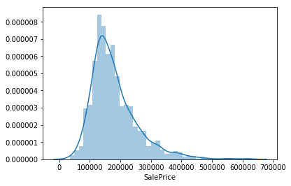
SalePrice deviates from a normal distribution and appears to be right-skewed. Linear models perform better with normally distributed data, so we should transform this variable. We can use the numpy.log1p() function to transform the data so that it is accurate for a wide range of floating point values. This is equivalent to ln(1+p), which allows us to include 0 values.

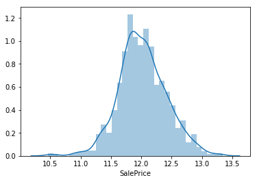
df_train['SalePrice'] = np.log1p(df_train['SalePrice'])

# Check the distribution again
sns.distplot(df_train['SalePrice']);

Correlation Heatmap

# Correlation map
corr = df_train.corr()
plt.subplots(figsize=(15,10))
sns.heatmap(corr, vmax=0.8, square=True)

<matplotlib.axes._subplots.AxesSubplot at 0x11c64a1d0>

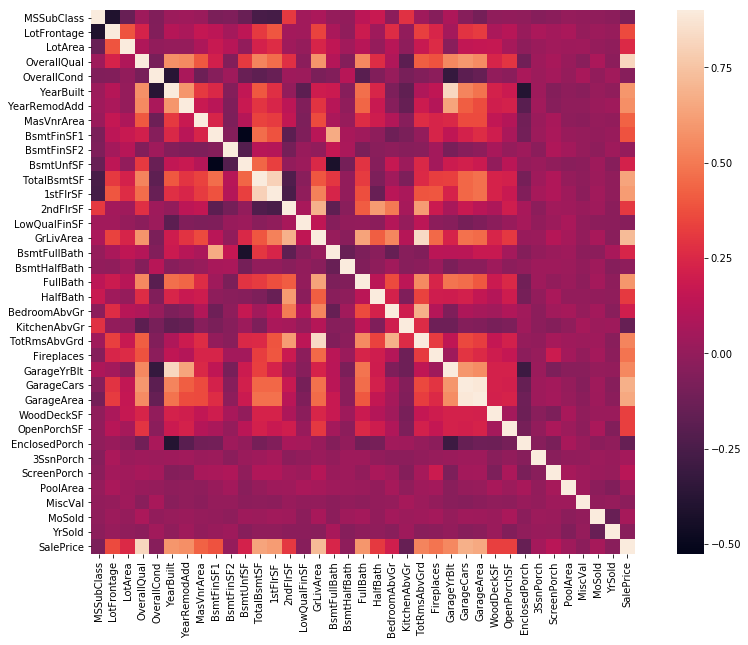
Most of the variables appear to be moderately correlated.

Feature Engineering

Handle Missing Values

We will impute the missing values for each feature. First, let’s see how many missing values there are.

# Missing data
total = df_train.isnull().sum().sort_values(ascending=False)
percent = (df_train.isnull().sum()/df_train.isnull().count()).sort_values(ascending=False)
missing_data = pd.concat([total, percent], axis=1, keys=['Total', 'Percent'])
missing_data.head(20)

	Total	Percent
PoolQC	1451	0.996566
MiscFeature	1402	0.962912
Alley	1365	0.937500
Fence	1176	0.807692
FireplaceQu	690	0.473901
LotFrontage	259	0.177885
GarageType	81	0.055632
GarageCond	81	0.055632
GarageFinish	81	0.055632
GarageQual	81	0.055632
GarageYrBlt	81	0.055632
BsmtFinType2	38	0.026099
BsmtExposure	38	0.026099
BsmtQual	37	0.025412
BsmtCond	37	0.025412
BsmtFinType1	37	0.025412
MasVnrArea	8	0.005495
MasVnrType	8	0.005495
Electrical	1	0.000687
RoofMatl	0	0.000000

PoolQC, MiscFeature, Alley, Fence, FireplaceQu

Since these features have a significant percentage of null values (>40%), we can safely just drop them entirely.

df_train = df_train.drop(['PoolQC', 'MiscFeature', 'Alley','Fence', 'FireplaceQu'], axis=1)

LotFrontage

We can assume that homes in the same neighborhood will have similar values for the linear feet of street connected to their property. Thus, we can use groupby to group according to neighborhood and fill in the missing values with the median LotFrontage.

df_train['LotFrontage'] = df_train.groupby('Neighborhood')['LotFrontage'].transform(lambda x: x.fillna(x.median()))
df_train['LotFrontage'].describe()

count    1456.000000
mean       69.895948
std        21.331035
min        21.000000
25%        60.000000
50%        70.000000
75%        80.000000
max       313.000000
Name: LotFrontage, dtype: float64

GarageType, GarageCond, GarageFinish, GarageQual, GarageYrBlt

For each of the categorical garage features, we can fill in the missing values with ‘None’, since it indicates no garage.

for col in ['GarageType', 'GarageFinish', 'GarageQual', 'GarageCond', 'GarageYrBlt']:
    df_train[col] = df_train[col].fillna('None')

BsmtQual, BsmtCond, BsmtFinType1

For these three basement features, we can fill in the missing values with ‘None’.

for col in ['BsmtQual', 'BsmtCond', 'BsmtFinType1']:
    df_train[col] = df_train[col].fillna('None')

BsmtFinType2, BsmtExposure

For these two basement features, we can fill in the missing values with ‘None’.

for col in ['BsmtFinType2', 'BsmtExposure']:
    df_train[col] = df_train[col].fillna('None')

MasVnrArea

A value of NaN means no masonry veneer for the home, so we can fill in missing values with 0.

df_train['MasVnrArea'] = df_train['MasVnrArea'].fillna(0)

MsVnrType

A value of NaN means no masonry veneer for the home, so we can fill in missing values with ‘None’.

df_train['MasVnrType'] = df_train['MasVnrType'].fillna('None')

Utilities

All of the values are ‘AllPub’ except for three of them. Therefore, this feature will not be useful for modeling, and we can safely drop it.

df_train = df_train.drop(['Utilities'], axis=1)

Functional

According to the data description, a value of NaN means typical. Thus, we can replace missing values with ‘Typ’.

df_train['Functional'] = df_train['Functional'].fillna('Typ')

Electrical

There is only one NaN value, so we can replace it with the most frequently occurring value, ‘SBrkr’.

df_train['Electrical'] = df_train['Electrical'].fillna(df_train['Electrical'].mode()[0])

# Check missing data
total = df_train.isnull().sum().sort_values(ascending=False)
percent = (df_train.isnull().sum()/df_train.isnull().count()).sort_values(ascending=False)
missing_data = pd.concat([total, percent], axis=1, keys=['Total', 'Percent'])
missing_data.head(19)

	Total	Percent
SalePrice	0	0.0
RoofStyle	0	0.0
Exterior1st	0	0.0
Exterior2nd	0	0.0
MasVnrType	0	0.0
MasVnrArea	0	0.0
ExterQual	0	0.0
ExterCond	0	0.0
Foundation	0	0.0
BsmtQual	0	0.0
BsmtCond	0	0.0
BsmtExposure	0	0.0
BsmtFinType1	0	0.0
BsmtFinSF1	0	0.0
BsmtFinType2	0	0.0
BsmtFinSF2	0	0.0
BsmtUnfSF	0	0.0
RoofMatl	0	0.0
YearRemodAdd	0	0.0

df_train.describe()

	MSSubClass	LotFrontage	LotArea	OverallQual	OverallCond	YearBuilt	YearRemodAdd	MasVnrArea	BsmtFinSF1	BsmtFinSF2	...	WoodDeckSF	OpenPorchSF	EnclosedPorch	3SsnPorch	ScreenPorch	PoolArea	MiscVal	MoSold	YrSold	SalePrice
count	1456.000000	1456.000000	1456.000000	1456.000000	1456.000000	1456.00000	1456.000000	1456.000000	1456.000000	1456.000000	...	1456.000000	1456.000000	1456.000000	1456.000000	1456.000000	1456.000000	1456.000000	1456.000000	1456.000000	1456.000000
mean	56.888736	69.895948	10448.784341	6.088599	5.576236	1971.18544	1984.819368	101.526786	436.991071	46.677198	...	93.833791	46.221154	22.014423	3.418956	15.102335	2.055632	43.608516	6.326236	2007.817308	12.021950
std	42.358363	21.331035	9860.763449	1.369669	1.113966	30.20159	20.652143	177.011773	430.255052	161.522376	...	125.192349	65.352424	61.192248	29.357056	55.828405	35.383772	496.799265	2.698356	1.329394	0.396077
min	20.000000	21.000000	1300.000000	1.000000	1.000000	1872.00000	1950.000000	0.000000	0.000000	0.000000	...	0.000000	0.000000	0.000000	0.000000	0.000000	0.000000	0.000000	1.000000	2006.000000	10.460271
25%	20.000000	60.000000	7538.750000	5.000000	5.000000	1954.00000	1966.750000	0.000000	0.000000	0.000000	...	0.000000	0.000000	0.000000	0.000000	0.000000	0.000000	0.000000	5.000000	2007.000000	11.774528
50%	50.000000	70.000000	9468.500000	6.000000	5.000000	1972.00000	1993.500000	0.000000	381.000000	0.000000	...	0.000000	24.000000	0.000000	0.000000	0.000000	0.000000	0.000000	6.000000	2008.000000	12.001512
75%	70.000000	80.000000	11588.000000	7.000000	6.000000	2000.00000	2004.000000	163.250000	706.500000	0.000000	...	168.000000	68.000000	0.000000	0.000000	0.000000	0.000000	0.000000	8.000000	2009.000000	12.273736
max	190.000000	313.000000	215245.000000	10.000000	9.000000	2010.00000	2010.000000	1600.000000	2188.000000	1474.000000	...	857.000000	547.000000	552.000000	508.000000	480.000000	738.000000	15500.000000	12.000000	2010.000000	13.345509

8 rows × 36 columns

Label Encoding Categorical Features

Since there are categorical features that depend on ordering (such as YrSold), we can encode all the categorical features using label encoding, which accounts for ordering.

# Convert some numerical features to categorical
for col in ['MSSubClass', 'OverallCond', 'YrSold', 'MoSold']:
    df_train[col] = df_train[col].apply(str)

print(df_train.dtypes)

MSSubClass         int64
MSZoning           int64
LotFrontage      float64
LotArea            int64
Street             int64
LotShape          object
LandContour       object
LotConfig         object
LandSlope         object
Neighborhood      object
Condition1        object
Condition2        object
BldgType          object
HouseStyle        object
OverallQual        int64
OverallCond       object
YearBuilt          int64
YearRemodAdd       int64
RoofStyle         object
RoofMatl          object
Exterior1st       object
Exterior2nd       object
MasVnrType        object
MasVnrArea       float64
ExterQual         object
ExterCond         object
Foundation        object
BsmtQual          object
BsmtCond          object
BsmtExposure      object
BsmtFinType1      object
BsmtFinSF1         int64
BsmtFinType2      object
BsmtFinSF2         int64
BsmtUnfSF          int64
TotalBsmtSF        int64
Heating           object
HeatingQC         object
CentralAir        object
Electrical        object
1stFlrSF           int64
2ndFlrSF           int64
LowQualFinSF       int64
GrLivArea          int64
BsmtFullBath       int64
BsmtHalfBath       int64
FullBath           int64
HalfBath           int64
BedroomAbvGr       int64
KitchenAbvGr       int64
KitchenQual       object
TotRmsAbvGrd       int64
Functional        object
Fireplaces         int64
GarageType        object
GarageYrBlt       object
GarageFinish      object
GarageCars         int64
GarageArea         int64
GarageQual        object
GarageCond        object
PavedDrive        object
WoodDeckSF         int64
OpenPorchSF        int64
EnclosedPorch      int64
3SsnPorch          int64
ScreenPorch        int64
PoolArea           int64
MiscVal            int64
MoSold            object
YrSold            object
SaleType          object
SaleCondition     object
SalePrice        float64
dtype: object

cols = ['MSSubClass', 'MSZoning', 'LotFrontage', 'Street', 'LotShape', 'LandContour', 'LotConfig',
        'LandSlope', 'Neighborhood', 'Condition1', 'Condition2', 'BldgType', 'HouseStyle', 'OverallCond', 'RoofStyle',
        'RoofMatl', 'Exterior1st', 'Exterior2nd', 'MasVnrType', 'MasVnrArea', 'ExterQual', 'ExterCond', 'Foundation',
        'BsmtQual', 'BsmtCond', 'BsmtExposure', 'BsmtFinType1', 'BsmtFinType2', 'Heating', 'HeatingQC', 'CentralAir',
        'Electrical', 'KitchenQual', 'Functional', 'GarageType', 'GarageYrBlt', 'GarageFinish', 'GarageQual',
        'GarageCond', 'PavedDrive', 'MoSold', 'YrSold', 'SaleType', 'SaleCondition']

# Apply LabelEncoder to categorical features
for col in cols:
    le = LabelEncoder() 
    le.fit(list(df_train[col].values)) 
    df_train[col] = le.transform(list(df_train[col].values))

Add TotalSF Feature

Let’s add a feature for the total square footage.

# Add feature for total square footage
df_train['TotalSF'] = df_train['TotalBsmtSF'] + df_train['1stFlrSF'] + df_train['2ndFlrSF']

Transform Skewed Features

In order to transform the features which deviate from a normal distribution, we must use a transformation. A log transformation is a possibility, but I decided to settle on the box-cox transformation, which is more flexible.

# Create a DataFrame of numerical features
numeric_features = df_train.dtypes[df_train.dtypes != 'object'].index

# Check the skew of numerical features
skewed_features = df_train[numeric_features].apply(lambda x: skew(x)).sort_values(ascending=False)
skewness = pd.DataFrame({'Skew': skewed_features})
skewness.head(10)

	Skew
MiscVal	24.418175
PoolArea	17.504556
Condition2	13.666839
LotArea	12.574590
3SsnPorch	10.279262
Heating	9.831083
LowQualFinSF	8.989291
RoofMatl	8.293646
LandSlope	4.801326
KitchenAbvGr	4.476748

# Include features that have a skewness greater than 0.75
skewness = skewness[abs(skewness) > 0.75]
print('Total skewed features: {}'.format(skewness.shape[0]))

skewed_features = skewness.index
alpha = 0.15
for feature in skewed_features:
    df_train[feature] = boxcox1p(df_train[feature], alpha)

Total skewed features: 75

# Convert categorical variable into dummy
df_train = pd.get_dummies(df_train)
df_train.head()

	MSSubClass	MSZoning	LotFrontage	LotArea	Street	LotShape	LandContour	LotConfig	LandSlope	Neighborhood	...	3SsnPorch	ScreenPorch	PoolArea	MiscVal	MoSold	YrSold	SaleType	SaleCondition	SalePrice	TotalSF
0	2.750250	1.540963	4.882973	19.212182	0.730463	1.540963	1.540963	1.820334	0.0	2.055642	...	0.0	0.0	0.0	0.0	1.820334	1.194318	2.602594	1.820334	3.156009	14.976591
1	1.820334	1.540963	5.527074	19.712205	0.730463	1.540963	1.540963	1.194318	0.0	4.137711	...	0.0	0.0	0.0	0.0	2.440268	0.730463	2.602594	1.820334	3.140516	14.923100
2	2.750250	1.540963	5.053371	20.347241	0.730463	0.000000	1.540963	1.820334	0.0	2.055642	...	0.0	0.0	0.0	0.0	3.011340	1.194318	2.602594	1.820334	3.163719	15.149678
3	2.885846	1.540963	4.545286	19.691553	0.730463	0.000000	1.540963	0.000000	0.0	2.259674	...	0.0	0.0	0.0	0.0	1.820334	0.000000	2.602594	0.000000	3.111134	14.857121
4	2.750250	1.540963	5.653921	21.325160	0.730463	0.000000	1.540963	1.194318	0.0	3.438110	...	0.0	0.0	0.0	0.0	1.540963	1.194318	2.602594	1.820334	3.176081	15.852312

5 rows × 75 columns

df_train.describe()

	MSSubClass	MSZoning	LotFrontage	LotArea	Street	LotShape	LandContour	LotConfig	LandSlope	Neighborhood	...	3SsnPorch	ScreenPorch	PoolArea	MiscVal	MoSold	YrSold	SaleType	SaleCondition	SalePrice	TotalSF
count	1456.000000	1456.000000	1456.000000	1456.000000	1456.000000	1456.000000	1456.000000	1456.000000	1456.000000	1456.000000	...	1456.000000	1456.000000	1456.000000	1456.000000	1456.000000	1456.000000	1456.000000	1456.000000	1456.000000	1456.000000
mean	2.120462	1.532216	4.838973	19.545432	0.727453	1.006929	1.439999	1.403936	0.043274	2.993064	...	0.131088	0.624309	0.036790	0.403946	2.211254	0.988608	2.478930	1.703198	3.130140	14.834646
std	0.804227	0.242085	1.198320	2.025558	0.046811	0.720319	0.338967	0.712903	0.186299	0.799155	...	1.023859	2.137374	0.627302	2.153524	0.740955	0.623489	0.465932	0.475669	0.044712	0.980603
min	0.000000	0.000000	0.000000	12.878993	0.000000	0.000000	0.000000	0.000000	0.000000	0.000000	...	0.000000	0.000000	0.000000	0.000000	0.000000	0.000000	0.000000	0.000000	2.944763	9.279836
25%	1.820334	1.540963	4.545286	18.773051	0.730463	0.000000	1.540963	1.194318	0.000000	2.440268	...	0.000000	0.000000	0.000000	0.000000	2.055642	0.730463	2.602594	1.820334	3.102566	14.195323
50%	2.055642	1.540963	5.133567	19.657692	0.730463	1.540963	1.540963	1.820334	0.000000	3.128239	...	0.000000	0.000000	0.000000	0.000000	2.440268	1.194318	2.602594	1.820334	3.128410	14.855815
75%	2.750250	1.540963	5.527074	20.467446	0.730463	1.540963	1.540963	1.820334	0.000000	3.618223	...	0.000000	0.000000	0.000000	0.000000	2.750250	1.540963	2.602594	1.820334	3.158902	15.488874
max	3.340760	1.820334	6.899104	35.391371	0.730463	1.540963	1.540963	1.820334	1.194318	4.137711	...	10.312501	10.169007	11.289160	21.677435	3.011340	1.820334	2.602594	2.055642	3.274014	18.172113

8 rows × 75 columns

Modeling

For our modeling, we will do three iterations:

• Full feature set
• Reduced feature set
• PCA

In each iteration, we will create five models:

• Linear Regression
• KNN Regression
• Random Forest Regresion
• Ridge Regression
• Lasso Regression

We will generate an accuracy score for each of the models and determine which model most accurately predicts our target variable, SalePrice. For iterations 1 and 2, we will use GridSearchCV to determine the best set of parameters for our model, and for iteration 3, we will use pipe to chain together PCA with our regression model.

X = df_train.drop(['SalePrice'], axis=1)
y = df_train.loc[:, ['SalePrice']]

X.head()

	MSSubClass	MSZoning	LotFrontage	LotArea	Street	LotShape	LandContour	LotConfig	LandSlope	Neighborhood	...	EnclosedPorch	3SsnPorch	ScreenPorch	PoolArea	MiscVal	MoSold	YrSold	SaleType	SaleCondition	TotalSF
0	2.750250	1.540963	4.882973	19.212182	0.730463	1.540963	1.540963	1.820334	0.0	2.055642	...	0.000000	0.0	0.0	0.0	0.0	1.820334	1.194318	2.602594	1.820334	14.976591
1	1.820334	1.540963	5.527074	19.712205	0.730463	1.540963	1.540963	1.194318	0.0	4.137711	...	0.000000	0.0	0.0	0.0	0.0	2.440268	0.730463	2.602594	1.820334	14.923100
2	2.750250	1.540963	5.053371	20.347241	0.730463	0.000000	1.540963	1.820334	0.0	2.055642	...	0.000000	0.0	0.0	0.0	0.0	3.011340	1.194318	2.602594	1.820334	15.149678
3	2.885846	1.540963	4.545286	19.691553	0.730463	0.000000	1.540963	0.000000	0.0	2.259674	...	8.797736	0.0	0.0	0.0	0.0	1.820334	0.000000	2.602594	0.000000	14.857121
4	2.750250	1.540963	5.653921	21.325160	0.730463	0.000000	1.540963	1.194318	0.0	3.438110	...	0.000000	0.0	0.0	0.0	0.0	1.540963	1.194318	2.602594	1.820334	15.852312

5 rows × 74 columns

X.describe()

	MSSubClass	MSZoning	LotFrontage	LotArea	Street	LotShape	LandContour	LotConfig	LandSlope	Neighborhood	...	EnclosedPorch	3SsnPorch	ScreenPorch	PoolArea	MiscVal	MoSold	YrSold	SaleType	SaleCondition	TotalSF
count	1456.000000	1456.000000	1456.000000	1456.000000	1456.000000	1456.000000	1456.000000	1456.000000	1456.000000	1456.000000	...	1456.000000	1456.000000	1456.000000	1456.000000	1456.000000	1456.000000	1456.000000	1456.000000	1456.000000	1456.000000
mean	2.120462	1.532216	4.838973	19.545432	0.727453	1.006929	1.439999	1.403936	0.043274	2.993064	...	1.041125	0.131088	0.624309	0.036790	0.403946	2.211254	0.988608	2.478930	1.703198	14.834646
std	0.804227	0.242085	1.198320	2.025558	0.046811	0.720319	0.338967	0.712903	0.186299	0.799155	...	2.589720	1.023859	2.137374	0.627302	2.153524	0.740955	0.623489	0.465932	0.475669	0.980603
min	0.000000	0.000000	0.000000	12.878993	0.000000	0.000000	0.000000	0.000000	0.000000	0.000000	...	0.000000	0.000000	0.000000	0.000000	0.000000	0.000000	0.000000	0.000000	0.000000	9.279836
25%	1.820334	1.540963	4.545286	18.773051	0.730463	0.000000	1.540963	1.194318	0.000000	2.440268	...	0.000000	0.000000	0.000000	0.000000	0.000000	2.055642	0.730463	2.602594	1.820334	14.195323
50%	2.055642	1.540963	5.133567	19.657692	0.730463	1.540963	1.540963	1.820334	0.000000	3.128239	...	0.000000	0.000000	0.000000	0.000000	0.000000	2.440268	1.194318	2.602594	1.820334	14.855815
75%	2.750250	1.540963	5.527074	20.467446	0.730463	1.540963	1.540963	1.820334	0.000000	3.618223	...	0.000000	0.000000	0.000000	0.000000	0.000000	2.750250	1.540963	2.602594	1.820334	15.488874
max	3.340760	1.820334	6.899104	35.391371	0.730463	1.540963	1.540963	1.820334	1.194318	4.137711	...	10.524981	10.312501	10.169007	11.289160	21.677435	3.011340	1.820334	2.602594	2.055642	18.172113

8 rows × 74 columns

y.head()

	SalePrice
0	3.156009
1	3.140516
2	3.163719
3	3.111134
4	3.176081

Iteration 1 - All Original Features

In this iteration, we will run our models with the full feature set.

# Split the data into train and test sets
X_train, X_test, y_train, y_test = train_test_split(X, y, test_size=0.2)

Linear Regression

# Instantiate model and create parameter grid
lr = linear_model.LinearRegression()
grid_params = {'fit_intercept': [True, False],
               'normalize': [True, False], 
               'copy_X' : [True, False]}

# Instantiate new grid
grid = GridSearchCV(lr, grid_params, n_jobs=-1, cv=5)

# Linear Regression
start = time.time()
grid.fit(X_train, y_train)
y_pred = grid.predict(X_test)
print('Runtime for grid search: {0:.3} s'.format((time.time() - start)))
print('Best Accuracy Score: \n{}'.format(grid.best_score_))
print('Best Parameters: \n{}'.format(grid.best_params_))

Runtime for grid search: 11.0 s
Best Accuracy Score: 
0.9038859588435272
Best Parameters: 
{'copy_X': True, 'fit_intercept': False, 'normalize': True}

# Instantiate and fit model with best parameters
lr = LinearRegression(fit_intercept=False, normalize=True, copy_X=True)
lr.fit(X_train, y_train)
y_pred = lr.predict(X_test)

# Run cross validation and calculate RMSE
scores = cross_val_score(lr, X_train, y_train, cv=5)

# Print results
print('Score With 20% Holdout:\n{0:.2%}'.format(lr.score(X_test, y_test)))
print('Cross Validation Scores:\n', scores)
print('Average Cross Validation Score:\n{0:.2%}'.format(scores.mean()))

# Calculate root mean squared error
rmse = mean_squared_error(np.expm1(y_test), np.expm1(y_pred))**0.5

# Print result
print('Root Mean Squared Error:\n{}'.format(rmse))

Score With 20% Holdout:
90.03%
Cross Validation Scores:
 [0.88870071 0.90088601 0.91468823 0.92236951 0.89273748]
Average Cross Validation Score:
90.39%
Root Mean Squared Error:
0.30628900378557106

KNN Regression

# Instantiate model and create parameter grid
knn = neighbors.KNeighborsRegressor()
grid_params = {'n_neighbors': list(range(1, 10)),
               'weights': ['uniform', 'distance'], 
               'algorithm' : ['auto', 'ball_tree', 'kd_tree', 'brute']}

# Instantiate new grid
grid = GridSearchCV(knn, grid_params, n_jobs=-1, cv=5)

# KNN Regression
start = time.time()
grid.fit(X_train, y_train)
y_pred = grid.predict(X_test)

# Print results
print('Runtime for grid search: {0:.3} s'.format((time.time() - start)))
print('Best Accuracy Score: \n{}'.format(grid.best_score_))
print('Best Parameters: \n{}'.format(grid.best_params_))

Runtime for grid search: 12.2 s
Best Accuracy Score: 
0.6595538969910677
Best Parameters: 
{'algorithm': 'brute', 'n_neighbors': 6, 'weights': 'distance'}

# Instantiate and fit model with best parameters
knn = neighbors.KNeighborsRegressor(n_neighbors=5, weights='distance', algorithm='auto')
knn.fit(X_train, y_train)
y_pred = knn.predict(X_test)

# Run cross validation and calculate RMSE
scores = cross_val_score(knn, X_train, y_train, cv=5)

# Print results
print('Score With 20% Holdout:\n{0:.2%}'.format(knn.score(X_test, y_test)))
print('Cross Validation Scores:\n', scores)
print('Average Cross Validation Score:\n{0:.2%}'.format(scores.mean()))

# Calculate root mean squared error
rmse = mean_squared_error(np.expm1(y_test), np.expm1(y_pred))**0.5

# Print result
print('Root Mean Squared Error:\n{}'.format(rmse))

Score With 20% Holdout:
62.46%
Cross Validation Scores:
 [0.64736072 0.64168616 0.65754486 0.67426629 0.65346698]
Average Cross Validation Score:
65.49%
Root Mean Squared Error:
0.612165517811808

Random Forest Regression

# Instantiate model and create parameter grid
rfr = RandomForestRegressor()
grid_params = {'n_estimators': list(range(1, 10)),
               'criterion': ['mse', 'mae'],
               'max_depth': list(range(1, 10))}

# Instantiate new grid
grid = GridSearchCV(rfr, grid_params, n_jobs=-1, cv=5)

# KNN Regression
start = time.time()
grid.fit(X_train, y_train)
y_pred = grid.predict(X_test)

# Print results
print('Runtime for grid search: {0:.3} s'.format((time.time() - start)))
print('Best Accuracy Score: \n{}'.format(grid.best_score_))
print('Best Parameters: \n{}'.format(grid.best_params_))

Runtime for grid search: 1.85e+02 s
Best Accuracy Score: 
0.8628202929561456
Best Parameters: 
{'criterion': 'mse', 'max_depth': 9, 'n_estimators': 8}


/Users/rakeshbhatia/anaconda/lib/python3.6/site-packages/sklearn/model_selection/_search.py:714: DataConversionWarning: A column-vector y was passed when a 1d array was expected. Please change the shape of y to (n_samples,), for example using ravel().
  self.best_estimator_.fit(X, y, **fit_params)

# Instantiate and fit model with best parameters
rfr = RandomForestRegressor(n_estimators=9, criterion='mse', max_depth=9)
rfr.fit(X_train, y_train.values.ravel())
y_pred = rfr.predict(X_test)

# Run cross validation and calculate RMSE
scores = cross_val_score(rfr, X_train, y_train.values.ravel(), cv=5)

# Print results
print('Score With 20% Holdout:\n{0:.2%}'.format(rfr.score(X_test, y_test.values.ravel())))
print('Cross Validation Scores:\n{}'.format(scores))
print('Average Cross Validation Score:\n{0:.2%}'.format(scores.mean()))

# Calculate root mean squared error
rmse = mean_squared_error(np.expm1(y_test), np.expm1(y_pred))**0.5

# Print result
print('Root Mean Squared Error:\n{}'.format(rmse))

Score With 20% Holdout:
85.10%
Cross Validation Scores:
[0.84404563 0.85909811 0.87318738 0.88366671 0.84070214]
Average Cross Validation Score:
86.01%
Root Mean Squared Error:
0.37838092392711603

Ridge Regression

# Instantiate model and create parameter grid
rr = Ridge()
grid_params = {'alpha': [0.0001, 0.001, 0.01, 0.1, 1, 5, 10, 25, 50, 100], 
               'fit_intercept': [True, False],
               'solver': ['cholesky', 'lsqr', 'sparse_cg']}
#               'solver': ['svd', 'cholesky', 'lsqr', 'sparse_cg', 'sag', 'saga']}

# Instantiate new grid
grid = GridSearchCV(rr, grid_params, n_jobs=-1, cv=5)

# Ridge Regression
start = time.time()
grid.fit(X_train, y_train)
y_pred = grid.predict(X_test)

# Print results
print('Runtime for grid search: {0:.3} s'.format((time.time() - start)))
print('Best Accuracy Score: \n{}'.format(grid.best_score_))
print('Best Parameters: \n{}'.format(grid.best_params_))

Runtime for grid search: 3.84 s
Best Accuracy Score: 
0.9047617389686792
Best Parameters: 
{'alpha': 1, 'fit_intercept': False, 'solver': 'cholesky'}

# Instantiate and fit model with best parameters
rr = Ridge(alpha=1, fit_intercept=False, solver='cholesky')
rr.fit(X_train, y_train)
y_pred = rr.predict(X_test)

# Run cross validation and calculate RMSE
scores = cross_val_score(rr, X_train, y_train, cv=5)

# Print results
print('Score With 20% Holdout:\n{0:.2%}'.format(rr.score(X_test, y_test)))
print('Cross Validation Scores:\n{}'.format(scores))
print('Average Cross Validation Score:\n{0:.2%}'.format(scores.mean()))

# Calculate root mean squared error
rmse = mean_squared_error(np.expm1(y_test), np.expm1(y_pred))**0.5

# Print result
print('Root Mean Squared Error:\n{}'.format(rmse))

Score With 20% Holdout:
90.06%
Cross Validation Scores:
[0.8875597  0.90103579 0.91604279 0.92492845 0.89419661]
Average Cross Validation Score:
90.48%
Root Mean Squared Error:
0.3062108626753103

Lasso Regression

# Instantiate model and create parameter grid
lasso = Lasso()
grid_params = {'alpha': [0.0001, 0.001, 0.01, 0.1, 1, 5, 10, 25, 50, 100], 
               'fit_intercept': [True, False],
               'max_iter': list(range(10))}
#               'solver': ['svd', 'cholesky', 'lsqr', 'sparse_cg', 'sag', 'saga']}

# Instantiate new grid
grid = GridSearchCV(lasso, grid_params, n_jobs=-1, cv=5)

# Ridge Regression
start = time.time()
grid.fit(X_train, y_train)
y_pred = grid.predict(X_test)

# Print results
print('Runtime for grid search: {0:.3} s'.format((time.time() - start)))
print('Best Accuracy Score: \n{}'.format(grid.best_score_))
print('Best Parameters: \n{}'.format(grid.best_params_))

Runtime for grid search: 11.0 s
Best Accuracy Score: 
0.8898671924495875
Best Parameters: 
{'alpha': 0.0001, 'fit_intercept': True, 'max_iter': 9}


/Users/rakeshbhatia/anaconda/lib/python3.6/site-packages/sklearn/model_selection/_search.py:813: DeprecationWarning: The default of the `iid` parameter will change from True to False in version 0.22 and will be removed in 0.24. This will change numeric results when test-set sizes are unequal.
  DeprecationWarning)
/Users/rakeshbhatia/anaconda/lib/python3.6/site-packages/sklearn/linear_model/coordinate_descent.py:475: ConvergenceWarning: Objective did not converge. You might want to increase the number of iterations. Duality gap: 0.13095565812133875, tolerance: 0.0002336781715295783
  positive)

# Instantiate and fit model with best parameters
lasso = Lasso(alpha=0.0001, fit_intercept=True, max_iter=9)
lasso.fit(X_train, y_train)
y_pred = rr.predict(X_test)

# Run cross validation and calculate RMSE
scores = cross_val_score(lasso, X_train, y_train, cv=5)

# Print results
print('Score With 20% Holdout:\n{0:.2%}'.format(rr.score(X_test, y_test)))
print('Cross Validation Scores:\n{}'.format(scores))
print('Average Cross Validation Score:\n{0:.2%}'.format(scores.mean()))

# Calculate root mean squared error
rmse = mean_squared_error(np.expm1(y_test), np.expm1(y_pred))**0.5

# Print result
print('Root Mean Squared Error:\n{}'.format(rmse))

Score With 20% Holdout:
90.06%
Cross Validation Scores:
[0.87973372 0.87451241 0.90024551 0.91381628 0.88098994]
Average Cross Validation Score:
88.99%
Root Mean Squared Error:
0.3062108626753103


/Users/rakeshbhatia/anaconda/lib/python3.6/site-packages/sklearn/linear_model/coordinate_descent.py:475: ConvergenceWarning: Objective did not converge. You might want to increase the number of iterations. Duality gap: 0.13095565812133875, tolerance: 0.0002336781715295783
  positive)
/Users/rakeshbhatia/anaconda/lib/python3.6/site-packages/sklearn/linear_model/coordinate_descent.py:475: ConvergenceWarning: Objective did not converge. You might want to increase the number of iterations. Duality gap: 0.10424985154274628, tolerance: 0.00019337793314266012
  positive)
/Users/rakeshbhatia/anaconda/lib/python3.6/site-packages/sklearn/linear_model/coordinate_descent.py:475: ConvergenceWarning: Objective did not converge. You might want to increase the number of iterations. Duality gap: 0.10145213039752624, tolerance: 0.0001859706045300572
  positive)
/Users/rakeshbhatia/anaconda/lib/python3.6/site-packages/sklearn/linear_model/coordinate_descent.py:475: ConvergenceWarning: Objective did not converge. You might want to increase the number of iterations. Duality gap: 0.10570657513985911, tolerance: 0.0001856118913612857
  positive)
/Users/rakeshbhatia/anaconda/lib/python3.6/site-packages/sklearn/linear_model/coordinate_descent.py:475: ConvergenceWarning: Objective did not converge. You might want to increase the number of iterations. Duality gap: 0.10555805840971894, tolerance: 0.00018213605478717467
  positive)
/Users/rakeshbhatia/anaconda/lib/python3.6/site-packages/sklearn/linear_model/coordinate_descent.py:475: ConvergenceWarning: Objective did not converge. You might want to increase the number of iterations. Duality gap: 0.1016345070657701, tolerance: 0.00018743708089921418
  positive)

Our best model in this iteration was Ridge Regression with an accuracy score of 90.06% and an RMSE of 0.30621.

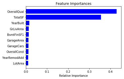
Iteration 2 - Feature Importances

In this iteration, we will use the feature importances from our Random Forest Regressor and extract the 20 most important features. Then, we will re-run all the models above on the reduced feature set.

features = X.columns
importances = rfr.feature_importances_
indices = np.argsort(importances)[-10:]  # top 10 features
plt.title('Feature Importances')
plt.barh(range(len(indices)), importances[indices], color='b', align='center')
plt.yticks(range(len(indices)), [features[i] for i in indices])
plt.xlabel('Relative Importance')
plt.show()

feature_importances = pd.DataFrame(rfr.feature_importances_, index = X.columns, 
                                   columns=['importance']).sort_values('importance',ascending=False)

feature_importances.head(20)

	importance
OverallQual	0.429685
TotalSF	0.355861
YearBuilt	0.015554
GrLivArea	0.013061
BsmtFinSF1	0.012794
GarageArea	0.011899
GarageCars	0.011873
OverallCond	0.011585
YearRemodAdd	0.011061
LotArea	0.010480
BsmtUnfSF	0.009619
CentralAir	0.009562
GarageYrBlt	0.006496
1stFlrSF	0.006414
GarageType	0.006077
Fireplaces	0.005345
LotFrontage	0.004462
2ndFlrSF	0.003897
SaleCondition	0.003872
Neighborhood	0.003725

X_reduced = X[['OverallQual', 'TotalSF', 'YearRemodAdd', 'GarageArea', 'CentralAir', 'GrLivArea', 
               'BsmtFinSF1', 'OverallCond', 'LotArea', 'GarageCond', 'YearBuilt', 'MSZoning', 
               '1stFlrSF', 'BsmtUnfSF', 'GarageType', 'GarageCars', 'BsmtFinType1', 'LotFrontage', 
               'BsmtQual', 'GarageYrBlt']]

X_reduced.head()

	OverallQual	TotalSF	YearRemodAdd	GarageArea	CentralAir	GrLivArea	BsmtFinSF1	OverallCond	LotArea	GarageCond	YearBuilt	MSZoning	1stFlrSF	BsmtUnfSF	GarageType	GarageCars	BsmtFinType1	LotFrontage	BsmtQual	GarageYrBlt
0	2.440268	14.976591	14.187527	10.506271	0.730463	13.698888	11.170327	1.820334	19.212182	2.055642	14.187527	1.540963	11.692623	7.483296	0.730463	1.194318	1.194318	4.882973	1.194318	6.426513
1	2.259674	14.923100	14.145138	10.062098	0.730463	12.792276	12.062832	2.440268	19.712205	2.055642	14.145138	1.540963	12.792276	8.897844	0.730463	1.194318	0.000000	5.527074	1.194318	5.744420
2	2.440268	15.149678	14.185966	10.775536	0.730463	13.832085	10.200343	1.820334	20.347241	2.055642	14.184404	1.540963	11.892039	9.917060	0.730463	1.194318	1.194318	5.053371	1.194318	6.382451
3	2.440268	14.857121	14.135652	10.918253	0.730463	13.711364	8.274266	1.820334	19.691553	2.055642	14.047529	1.540963	12.013683	10.468500	2.055642	1.540963	0.000000	4.545286	1.820334	6.314735
4	2.602594	15.852312	14.182841	11.627708	0.730463	14.480029	10.971129	1.820334	21.325160	2.055642	14.182841	1.540963	12.510588	10.221051	0.730463	1.540963	1.194318	5.653921	1.194318	6.360100

X_train, X_test, y_train, y_test = train_test_split(X_reduced, y, test_size=0.2)

Linear Regression

# Instantiate model and create parameter grid
lr = linear_model.LinearRegression()
grid_params = {'fit_intercept': [True, False],
               'normalize': [True, False], 
               'copy_X' : [True, False]}

# Instantiate new grid
grid = GridSearchCV(lr, grid_params, n_jobs=-1, cv=5)

# Linear Regression
start = time.time()
grid.fit(X_train, y_train)
y_pred = grid.predict(X_test)
print('Runtime for grid search: {0:.3} s'.format((time.time() - start)))
print('Best Accuracy Score: \n{}'.format(grid.best_score_))
print('Best Parameters: \n{}'.format(grid.best_params_))

Runtime for grid search: 0.568 s
Best Accuracy Score: 
0.8815714122815158
Best Parameters: 
{'copy_X': True, 'fit_intercept': True, 'normalize': False}

# Instantiate and fit model with best parameters
lr = LinearRegression(fit_intercept=False, normalize=True, copy_X=True)
lr.fit(X_train, y_train)
y_pred = lr.predict(X_test)

# Run cross validation and calculate RMSE
scores = cross_val_score(lr, X_train, y_train, cv=5)

# Print results
print('Score With 20% Holdout:\n{0:.2%}'.format(lr.score(X_test, y_test)))
print('Cross Validation Scores:\n', scores)
print('Average Cross Validation Score:\n{0:.2%}'.format(scores.mean()))

# Calculate root mean squared error
rmse = mean_squared_error(np.expm1(y_test), np.expm1(y_pred))**0.5

# Print result
print('Root Mean Squared Error:\n{}'.format(rmse))

Score With 20% Holdout:
91.45%
Cross Validation Scores:
 [0.86964536 0.90312406 0.87734731 0.86610569 0.88772752]
Average Cross Validation Score:
88.08%
Root Mean Squared Error:
0.3011926609631838

KNN Regression

# Instantiate model and create parameter grid
knn = neighbors.KNeighborsRegressor()
grid_params = {'n_neighbors': list(range(1, 10)),
               'weights': ['uniform', 'distance'], 
               'algorithm' : ['auto', 'ball_tree', 'kd_tree', 'brute']}

# Instantiate new grid
grid = GridSearchCV(knn, grid_params, n_jobs=-1, cv=5)

# KNN Regression
start = time.time()
grid.fit(X_train, y_train)
y_pred = grid.predict(X_test)

# Print results
print('Runtime for grid search: {0:.3} s'.format((time.time() - start)))
print('Best Accuracy Score: \n{}'.format(grid.best_score_))
print('Best Parameters: \n{}'.format(grid.best_params_))

Runtime for grid search: 4.46 s
Best Accuracy Score: 
0.7573965453742735
Best Parameters: 
{'algorithm': 'auto', 'n_neighbors': 7, 'weights': 'distance'}

# Instantiate and fit model with best parameters
knn = neighbors.KNeighborsRegressor(n_neighbors=7, weights='distance', algorithm='auto')
knn.fit(X_train, y_train)
y_pred = knn.predict(X_test)

# Run cross validation and calculate RMSE
scores = cross_val_score(knn, X_train, y_train, cv=5)

# Print results
print('Score With 20% Holdout:\n{0:.2%}'.format(knn.score(X_test, y_test)))
print('Cross Validation Scores:\n', scores)
print('Average Cross Validation Score:\n{0:.2%}'.format(scores.mean()))

# Calculate root mean squared error
rmse = mean_squared_error(np.expm1(y_test), np.expm1(y_pred))**0.5

# Print result
print('Root Mean Squared Error:\n{}'.format(rmse))

Score With 20% Holdout:
80.35%
Cross Validation Scores:
 [0.7559988  0.81061274 0.72753457 0.75354858 0.73920998]
Average Cross Validation Score:
75.74%
Root Mean Squared Error:
0.4564285807903383

Random Forest Regression

# Instantiate model and create parameter grid
rfr = RandomForestRegressor()
grid_params = {'n_estimators': list(range(1, 10)),
               'criterion': ['mse', 'mae'],
               'max_depth': list(range(1, 10))}

# Instantiate new grid
grid = GridSearchCV(rfr, grid_params, n_jobs=-1, cv=5)

# KNN Regression
start = time.time()
grid.fit(X_train, y_train)
y_pred = grid.predict(X_test)

# Print results
print('Runtime for grid search: {0:.3} s'.format((time.time() - start)))
print('Best Accuracy Score: \n{}'.format(grid.best_score_))
print('Best Parameters: \n{}'.format(grid.best_params_))

Runtime for grid search: 70.4 s
Best Accuracy Score: 
0.8517071234529742
Best Parameters: 
{'criterion': 'mse', 'max_depth': 9, 'n_estimators': 8}


/Users/rakeshbhatia/anaconda/lib/python3.6/site-packages/sklearn/model_selection/_search.py:714: DataConversionWarning: A column-vector y was passed when a 1d array was expected. Please change the shape of y to (n_samples,), for example using ravel().
  self.best_estimator_.fit(X, y, **fit_params)

# Instantiate and fit model with best parameters
rfr = RandomForestRegressor(n_estimators=9, criterion='mse', max_depth=8)
rfr.fit(X_train, y_train.values.ravel())
y_pred = rfr.predict(X_test)

# Run cross validation and calculate RMSE
scores = cross_val_score(rfr, X_train, y_train.values.ravel(), cv=5)

# Print results
print('Score With 20% Holdout:\n{0:.2%}'.format(rfr.score(X_test, y_test.values.ravel())))
print('Cross Validation Scores:\n{}'.format(scores))
print('Average Cross Validation Score:\n{0:.2%}'.format(scores.mean()))

# Calculate root mean squared error
rmse = mean_squared_error(np.expm1(y_test), np.expm1(y_pred))**0.5

# Print result
print('Root Mean Squared Error:\n{}'.format(rmse))

Score With 20% Holdout:
87.90%
Cross Validation Scores:
[0.84591098 0.86758539 0.85590976 0.82783851 0.84731086]
Average Cross Validation Score:
84.89%
Root Mean Squared Error:
0.3571122712911688

Ridge Regression

# Instantiate model and create parameter grid
rr = Ridge()
grid_params = {'alpha': [0.0001, 0.001, 0.01, 0.1, 1, 5, 10, 25, 50, 100], 
               'fit_intercept': [True, False],
               'solver': ['cholesky', 'lsqr', 'sparse_cg']}
#               'solver': ['svd', 'cholesky', 'lsqr', 'sparse_cg', 'sag', 'saga']}

# Instantiate new grid
grid = GridSearchCV(rr, grid_params, n_jobs=-1, cv=5)

# Ridge Regression
start = time.time()
grid.fit(X_train, y_train)
y_pred = grid.predict(X_test)

# Print results
print('Runtime for grid search: {0:.3} s'.format((time.time() - start)))
print('Best Accuracy Score: \n{}'.format(grid.best_score_))
print('Best Parameters: \n{}'.format(grid.best_params_))

Runtime for grid search: 2.3 s
Best Accuracy Score: 
0.8816035431498964
Best Parameters: 
{'alpha': 0.01, 'fit_intercept': True, 'solver': 'cholesky'}


/Users/rakeshbhatia/anaconda/lib/python3.6/site-packages/sklearn/model_selection/_search.py:813: DeprecationWarning: The default of the `iid` parameter will change from True to False in version 0.22 and will be removed in 0.24. This will change numeric results when test-set sizes are unequal.
  DeprecationWarning)

# Instantiate and fit model with best parameters
rr = Ridge(alpha=0.01, fit_intercept=True, solver='cholesky')
rr.fit(X_train, y_train)
y_pred = rr.predict(X_test)

# Run cross validation and calculate RMSE
scores = cross_val_score(rr, X_train, y_train, cv=5)

# Print results
print('Score With 20% Holdout:\n{0:.2%}'.format(rr.score(X_test, y_test)))
print('Cross Validation Scores:\n{}'.format(scores))
print('Average Cross Validation Score:\n{0:.2%}'.format(scores.mean()))

# Calculate root mean squared error
rmse = mean_squared_error(np.expm1(y_test), np.expm1(y_pred))**0.5

# Print result
print('Root Mean Squared Error:\n{}'.format(rmse))

Score With 20% Holdout:
90.10%
Cross Validation Scores:
[0.90876598 0.91318546 0.89388285 0.88931054 0.8936684 ]
Average Cross Validation Score:
89.98%
Root Mean Squared Error:
0.3149498700624098

Lasso Regression

# Instantiate model and create parameter grid
lasso = Lasso()
grid_params = {'alpha': [0.0001, 0.001, 0.01, 0.1, 1, 5, 10, 25, 50, 100], 
               'fit_intercept': [True, False],
               'max_iter': list(range(10))}
#               'solver': ['svd', 'cholesky', 'lsqr', 'sparse_cg', 'sag', 'saga']}

# Instantiate new grid
grid = GridSearchCV(lasso, grid_params, n_jobs=-1, cv=5)

# Ridge Regression
start = time.time()
grid.fit(X_train, y_train)
y_pred = grid.predict(X_test)

# Print results
print('Runtime for grid search: {0:.3} s'.format((time.time() - start)))
print('Best Accuracy Score: \n{}'.format(grid.best_score_))
print('Best Parameters: \n{}'.format(grid.best_params_))

Runtime for grid search: 8.92 s
Best Accuracy Score: 
0.8717199839344799
Best Parameters: 
{'alpha': 0.0001, 'fit_intercept': True, 'max_iter': 9}


/Users/rakeshbhatia/anaconda/lib/python3.6/site-packages/sklearn/model_selection/_search.py:813: DeprecationWarning: The default of the `iid` parameter will change from True to False in version 0.22 and will be removed in 0.24. This will change numeric results when test-set sizes are unequal.
  DeprecationWarning)
/Users/rakeshbhatia/anaconda/lib/python3.6/site-packages/sklearn/linear_model/coordinate_descent.py:475: ConvergenceWarning: Objective did not converge. You might want to increase the number of iterations. Duality gap: 0.1345447112339042, tolerance: 0.0002292111729539456
  positive)

# Instantiate and fit model with best parameters
lasso = Lasso(alpha=0.0001, fit_intercept=True, max_iter=9)
lasso.fit(X_train, y_train)
y_pred = rr.predict(X_test)

# Run cross validation and calculate RMSE
scores = cross_val_score(lasso, X_train, y_train, cv=5)

# Print results
print('Score With 20% Holdout:\n{0:.2%}'.format(rr.score(X_test, y_test)))
print('Cross Validation Scores:\n{}'.format(scores))
print('Average Cross Validation Score:\n{0:.2%}'.format(scores.mean()))

# Calculate root mean squared error
rmse = mean_squared_error(np.expm1(y_test), np.expm1(y_pred))**0.5

# Print result
print('Root Mean Squared Error:\n{}'.format(rmse))

Score With 20% Holdout:
90.10%
Cross Validation Scores:
[0.90610849 0.89638496 0.88806663 0.87695657 0.88558265]
Average Cross Validation Score:
89.06%
Root Mean Squared Error:
0.3149498700624098


/Users/rakeshbhatia/anaconda/lib/python3.6/site-packages/sklearn/linear_model/coordinate_descent.py:475: ConvergenceWarning: Objective did not converge. You might want to increase the number of iterations. Duality gap: 0.12588123641539328, tolerance: 0.000230805802977206
  positive)
/Users/rakeshbhatia/anaconda/lib/python3.6/site-packages/sklearn/linear_model/coordinate_descent.py:475: ConvergenceWarning: Objective did not converge. You might want to increase the number of iterations. Duality gap: 0.10174824166285584, tolerance: 0.00018211493454537317
  positive)
/Users/rakeshbhatia/anaconda/lib/python3.6/site-packages/sklearn/linear_model/coordinate_descent.py:475: ConvergenceWarning: Objective did not converge. You might want to increase the number of iterations. Duality gap: 0.10071330950203666, tolerance: 0.00018551750660764676
  positive)
/Users/rakeshbhatia/anaconda/lib/python3.6/site-packages/sklearn/linear_model/coordinate_descent.py:475: ConvergenceWarning: Objective did not converge. You might want to increase the number of iterations. Duality gap: 0.09815849040592911, tolerance: 0.00018381355085247963
  positive)
/Users/rakeshbhatia/anaconda/lib/python3.6/site-packages/sklearn/linear_model/coordinate_descent.py:475: ConvergenceWarning: Objective did not converge. You might want to increase the number of iterations. Duality gap: 0.10004544276933801, tolerance: 0.00018724225322712702
  positive)
/Users/rakeshbhatia/anaconda/lib/python3.6/site-packages/sklearn/linear_model/coordinate_descent.py:475: ConvergenceWarning: Objective did not converge. You might want to increase the number of iterations. Duality gap: 0.0976469770913432, tolerance: 0.00018434117216229712
  positive)

Our best model in this iteration was Linear Regression with an accuracy score of 91.45% and an RMSE of 0.30119.

Iteration 3 - PCA

In this iteration, we will use PCA to reduce our feature set and then run the same five models again.

Train and Test PCA

X_train, X_test, y_train, y_test = train_test_split(X, y, test_size=0.2)

# Standardize features
X_scaler = StandardScaler().fit_transform(X_train)

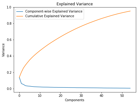
# Create PCA that retains 95% of variance
pca = PCA(n_components=0.95, whiten=True)

# Generate PCA
X_pca = pca.fit_transform(X_scaler)

# Print results
print('Original number of features:', X.shape[1])
print('Reduced number of features:', X_pca.shape[1])

Original number of features: 74
Reduced number of features: 55

fig = plt.figure(figsize=(7,5))
ax = plt.subplot(111)
ax.plot(range(X_pca.shape[1]), pca.explained_variance_ratio_, label='Component-wise Explained Variance')
ax.plot(range(X_pca.shape[1]), np.cumsum(pca.explained_variance_ratio_), label='Cumulative Explained Variance')
plt.title('Explained Variance')
plt.xlabel('Components')
plt.ylabel('Variance')
ax.legend()
plt.show()

Linear Regression

lr = linear_model.LinearRegression()
pipe = Pipeline([('pca', pca), ('linear', lr)])
pipe.fit(X_train, y_train)
y_pred = pipe.predict(X_test)

scores_train = cross_val_score(pipe, X_train, y_train, cv=5)
scores_test = cross_val_score(pipe, X_test, y_test, cv=5)
print('Cross Validation Scores - Training Set: \n{}'.format(scores_train))
print('\nAverage Cross Validation Score - Training Set: \n{:.2%}'.format(scores_train.mean()))
print('\nCross Validation Scores - Test Set: \n{}'.format(scores_train))
print('\nAverage Cross Validation Score - Test Set: \n{:.2%}'.format(scores_test.mean()))

# Calculate root mean squared error
rmse = mean_squared_error(np.expm1(y_test), np.expm1(y_pred))**0.5

# Print result
print('Root Mean Squared Error:\n{}'.format(rmse))

Cross Validation Scores - Training Set: 
[0.87208941 0.84418757 0.7806751  0.8441039  0.86005551]

Average Cross Validation Score - Training Set: 
84.02%

Cross Validation Scores - Test Set: 
[0.87208941 0.84418757 0.7806751  0.8441039  0.86005551]

Average Cross Validation Score - Test Set: 
72.61%
Root Mean Squared Error:
0.4570210334553902

KNN Regression

knn = neighbors.KNeighborsRegressor(n_neighbors=7, weights='distance', algorithm='auto')
pipe = Pipeline([('pca', pca), ('knn', knn)])
pipe.fit(X_train, y_train)
y_pred = pipe.predict(X_test)

scores_train = cross_val_score(pipe, X_train, y_train, cv=5)
scores_test = cross_val_score(pipe, X_test, y_test, cv=5)
print('Cross Validation Scores - Training Set: \n{}'.format(scores_train))
print('\nAverage Cross Validation Score - Training Set: \n{:.2%}'.format(scores_train.mean()))
print('\nCross Validation Scores - Test Set: \n{}'.format(scores_train))
print('\nAverage Cross Validation Score - Test Set: \n{:.2%}'.format(scores_test.mean()))

# Calculate root mean squared error
rmse = mean_squared_error(np.expm1(y_test), np.expm1(y_pred))**0.5

# Print result
print('Root Mean Squared Error:\n{}'.format(rmse))

Cross Validation Scores - Training Set: 
[0.72190707 0.6670871  0.63802632 0.59866867 0.68857193]

Average Cross Validation Score - Training Set: 
66.29%

Cross Validation Scores - Test Set: 
[0.72190707 0.6670871  0.63802632 0.59866867 0.68857193]

Average Cross Validation Score - Test Set: 
53.20%
Root Mean Squared Error:
0.608803837051414

Random Forest Regression

rfr = RandomForestRegressor(n_estimators=9, criterion='mse', max_depth=8)
pipe = Pipeline([('pca', pca), ('rfr', rfr)])
pipe.fit(X_train, y_train.values.ravel())
y_pred = pipe.predict(X_test)

scores_train = cross_val_score(pipe, X_train, y_train.values.ravel(), cv=5)
scores_test = cross_val_score(pipe, X_test, y_test.values.ravel(), cv=5)
print('Cross Validation Scores - Training Set: \n{}'.format(scores_train))
print('\nAverage Cross Validation Score - Training Set: \n{:.2%}'.format(scores_train.mean()))
print('\nCross Validation Scores - Test Set: \n{}'.format(scores_train))
print('\nAverage Cross Validation Score - Test Set: \n{:.2%}'.format(scores_test.mean()))

# Calculate root mean squared error
rmse = mean_squared_error(np.expm1(y_test), np.expm1(y_pred))**0.5

# Print result
print('Root Mean Squared Error:\n{}'.format(rmse))

Cross Validation Scores - Training Set: 
[0.77341358 0.69389058 0.67620675 0.70998848 0.77364554]

Average Cross Validation Score - Training Set: 
72.54%

Cross Validation Scores - Test Set: 
[0.77341358 0.69389058 0.67620675 0.70998848 0.77364554]

Average Cross Validation Score - Test Set: 
59.05%
Root Mean Squared Error:
0.5319618143549292

Ridge Regression

rr = Ridge()
pipe = Pipeline([('pca', pca), ('ridge', rr)])
pipe.fit(X_train, y_train)
y_pred = pipe.predict(X_test)

scores_train = cross_val_score(pipe, X_train, y_train, cv=5)
scores_test = cross_val_score(pipe, X_test, y_test, cv=5)
print('Cross Validation Scores - Training Set: \n{}'.format(scores_train))
print('\nAverage Cross Validation Score - Training Set: \n{:.2%}'.format(scores_train.mean()))
print('\nCross Validation Scores - Test Set: \n{}'.format(scores_train))
print('\nAverage Cross Validation Score - Test Set: \n{:.2%}'.format(scores_test.mean()))

# Calculate root mean squared error
rmse = mean_squared_error(np.expm1(y_test), np.expm1(y_pred))**0.5

# Print result
print('Root Mean Squared Error:\n{}'.format(rmse))

Cross Validation Scores - Training Set: 
[0.8721049  0.84420952 0.78061565 0.84410179 0.86007169]

Average Cross Validation Score - Training Set: 
84.02%

Cross Validation Scores - Test Set: 
[0.8721049  0.84420952 0.78061565 0.84410179 0.86007169]

Average Cross Validation Score - Test Set: 
72.65%
Root Mean Squared Error:
0.4570192792436453

Lasso Regression

lasso = Lasso(alpha=0.0001, fit_intercept=True, max_iter=9)
pipe = Pipeline([('pca', pca), ('lasso', lasso)])
pipe.fit(X_train, y_train)
y_pred = pipe.predict(X_test)

scores_train = cross_val_score(pipe, X_train, y_train, cv=5)
scores_test = cross_val_score(pipe, X_test, y_test, cv=5)
print('Cross Validation Scores - Training Set: \n{}'.format(scores_train))
print('\nAverage Cross Validation Score - Training Set: \n{:.2%}'.format(scores_train.mean()))
print('\nCross Validation Scores - Test Set: \n{}'.format(scores_train))
print('\nAverage Cross Validation Score - Test Set: \n{:.2%}'.format(scores_test.mean()))

# Calculate root mean squared error
rmse = mean_squared_error(np.expm1(y_test), np.expm1(y_pred))**0.5

# Print result
print('Root Mean Squared Error:\n{}'.format(rmse))

Cross Validation Scores - Training Set: 
[0.87197939 0.84464882 0.78050591 0.84374574 0.85970556]

Average Cross Validation Score - Training Set: 
84.01%

Cross Validation Scores - Test Set: 
[0.87197939 0.84464882 0.78050591 0.84374574 0.85970556]

Average Cross Validation Score - Test Set: 
72.66%
Root Mean Squared Error:
0.45644992470380247

Our best model in this iteration was Lasso Regression with an average cross validation score (test set) of 72.66% and an RMSE of 0.45645.

Conclusion

Overall, the first two iterations appeared to provide the best results. There was even a slight improvement in some of the models from iteration 1 to iteration 2, when we limited the feature set to the 20 most important features. However, there was a significant drop-off when we used a PCA that retained 95% of the variance. Thus, utilizing the feature importances appears to be most optimal way to model this dataset.