Data Science Portfolio
Plotting S-parameter Distributions with Matplotlib
import csv
import string
import numpy
import pandas as pd
import matplotlib.pyplot as plt
1804A Data
df = pd.read_csv('docs/F123019_1_B18U01_BST1804A_S_full.csv', delimiter='\;')
df = df.drop(['XAdress', 'YAdress', 'PhS11', 'dBS12', 'PhS12', 'PhS21', 'PhS22', 'Unnamed: 11'], axis=1).dropna()
df.head()
/Users/rakeshbhatia/anaconda/lib/python3.6/site-packages/ipykernel_launcher.py:1: ParserWarning: Falling back to the 'python' engine because the 'c' engine does not support regex separators (separators > 1 char and different from '\s+' are interpreted as regex); you can avoid this warning by specifying engine='python'.
  """Entry point for launching an IPython kernel.
| Freq | dBS11 | dBS21 | dBS22 | |
|---|---|---|---|---|
| 0 | 0.1 | -5.376231 | 8.581573 | -1.337611 |
| 1 | 0.2 | -9.890681 | 13.300380 | -4.357149 |
| 2 | 0.3 | -11.544020 | 15.064870 | -7.260980 |
| 3 | 0.4 | -13.141930 | 16.082660 | -9.876349 |
| 4 | 0.5 | -14.926210 | 16.647800 | -11.990410 |
print(df.dtypes)
Freq     float64
dBS11    float64
dBS21    float64
dBS22    float64
dtype: object
Extract 0.5GHz Data
# Extract only the data for Freq = 0.5
df1 = df.loc[df['Freq'] == 0.5]
df1.head()
| Freq | dBS11 | dBS21 | dBS22 | |
|---|---|---|---|---|
| 4 | 0.5 | -14.92621 | 16.64780 | -11.99041 |
| 404 | 0.5 | -14.97190 | 16.74654 | -11.86176 |
| 804 | 0.5 | -14.95612 | 16.69878 | -11.91722 |
| 1204 | 0.5 | -14.22709 | 16.38852 | -11.07036 |
| 1604 | 0.5 | -14.96282 | 16.70663 | -11.84028 |
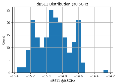
dBS11 Distribution (0.5GHz)
# Plot dBS11 distribution at 0.5GHz
df1.dBS11.hist(bins=20)
plt.title('dBS11 Distribution @0.5GHz')
plt.xlabel('dBS11 @0.5GHz')
plt.ylabel('Count')
plt.show()
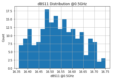
dBS21 Distribution (0.5GHz)
# Plot dBS21 distribution at 0.5GHz
df1.dBS21.hist(bins=20)
plt.title('dBS11 Distribution @0.5GHz')
plt.xlabel('dBS11 @0.5GHz')
plt.ylabel('Count')
plt.show()
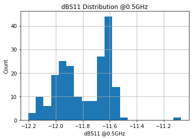
dBS22 Distribution (0.5GHz)
# Plot dBS22 distribution at 0.5GHz
df1.dBS22.hist(bins=20)
plt.title('dBS11 Distribution @0.5GHz')
plt.xlabel('dBS11 @0.5GHz')
plt.ylabel('Count')
plt.show()
Key Statistics (Freq=0.5GHz)
df1.describe()
| Freq | dBS11 | dBS21 | dBS22 | |
|---|---|---|---|---|
| count | 199.0 | 199.000000 | 199.000000 | 199.000000 |
| mean | 0.5 | -14.903008 | 16.537706 | -11.794446 |
| std | 0.0 | 0.205054 | 0.095247 | 0.186803 |
| min | 0.5 | -15.368250 | 16.360120 | -12.204510 |
| 25% | 0.5 | -15.068910 | 16.469755 | -11.950350 |
| 50% | 0.5 | -14.903110 | 16.532240 | -11.787360 |
| 75% | 0.5 | -14.750420 | 16.607040 | -11.627005 |
| max | 0.5 | -14.227090 | 16.750850 | -11.070360 |
Extract 6GHz Data
# Extract only the data for Freq = 6
df2 = df.loc[df['Freq'] == 6]
df2.head()
| Freq | dBS11 | dBS21 | dBS22 | |
|---|---|---|---|---|
| 59 | 6.0 | -10.028930 | 16.62984 | -12.40061 |
| 459 | 6.0 | -10.172090 | 16.72707 | -12.06172 |
| 859 | 6.0 | -10.108140 | 16.67642 | -12.20471 |
| 1259 | 6.0 | -8.866876 | 15.76777 | -15.91539 |
| 1659 | 6.0 | -10.150780 | 16.67780 | -12.19041 |
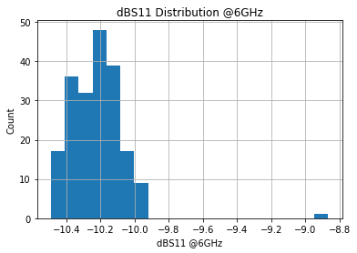
dBS11 Distribution (6GHz)
# Plot dBS11 distribution at 6GHz
df2.dBS11.hist(bins=20)
plt.title('dBS11 Distribution @6GHz')
plt.xlabel('dBS11 @6GHz')
plt.ylabel('Count')
plt.show()
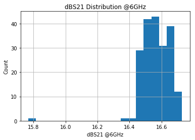
dBS21 Distribution (6GHz)
# Plot dBS21 distribution at 6GHz
df2.dBS21.hist(bins=20)
plt.title('dBS21 Distribution @6GHz')
plt.xlabel('dBS21 @6GHz')
plt.ylabel('Count')
plt.show()
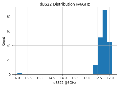
dBS22 Distribution (6GHz)
# Plot dBS22 distribution at 6GHz
df2.dBS22.hist(bins=20)
plt.title('dBS22 Distribution @6GHz')
plt.xlabel('dBS22 @6GHz')
plt.ylabel('Count')
plt.show()
Key Statistics (Freq=6GHz)
df2.describe()
| Freq | dBS11 | dBS21 | dBS22 | |
|---|---|---|---|---|
| count | 199.0 | 199.000000 | 199.000000 | 199.000000 |
| mean | 6.0 | -10.223419 | 16.565023 | -12.234007 |
| std | 0.0 | 0.160035 | 0.092270 | 0.308394 |
| min | 6.0 | -10.489480 | 15.767770 | -15.915390 |
| 25% | 6.0 | -10.330915 | 16.503145 | -12.325785 |
| 50% | 6.0 | -10.217370 | 16.563700 | -12.212220 |
| 75% | 6.0 | -10.139460 | 16.633205 | -12.093165 |
| max | 6.0 | -8.866876 | 16.727920 | -11.880080 |
Extract 9GHz Data
# Extract only the data for Freq = 9
df3 = df.loc[df['Freq'] == 8.999999]
df3.head()
| Freq | dBS11 | dBS21 | dBS22 | |
|---|---|---|---|---|
| 89 | 8.999999 | -12.405270 | 17.76468 | -10.140230 |
| 489 | 8.999999 | -12.667990 | 17.85854 | -9.749912 |
| 889 | 8.999999 | -12.583610 | 17.79932 | -9.957961 |
| 1289 | 8.999999 | -9.918789 | 15.61766 | -9.632690 |
| 1689 | 8.999999 | -12.679570 | 17.79396 | -9.940454 |
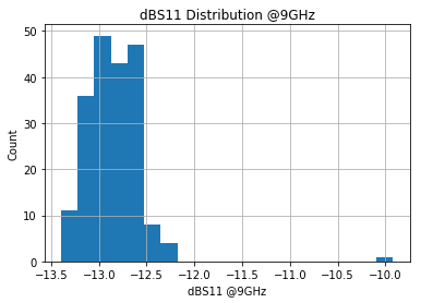
dBS11 Distribution (9GHz)
# Plot dBS11 distribution at 9GHz
df3.dBS11.hist(bins=20)
plt.title('dBS11 Distribution @9GHz')
plt.xlabel('dBS11 @9GHz')
plt.ylabel('Count')
plt.show()
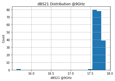
dBS21 Distribution (9GHz)
# Plot dBS21 distribution at 9GHz
df3.dBS21.hist(bins=20)
plt.title('dBS21 Distribution @9GHz')
plt.xlabel('dBS21 @9GHz')
plt.ylabel('Count')
plt.show()
dBS22 Distribution (9GHz)
# Plot dBS22 distribution at 9GHz
df3.dBS22.hist(bins=20)
plt.title('dBS22 Distribution @9GHz')
plt.xlabel('dBS22 @9GHz')
plt.ylabel('Count')
plt.show()
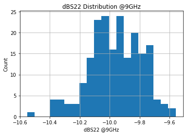
Key Statistics (Freq=9GHz)
df3.describe()
| Freq | dBS11 | dBS21 | dBS22 | |
|---|---|---|---|---|
| count | 1.990000e+02 | 199.000000 | 199.000000 | 199.000000 |
| mean | 8.999999e+00 | -12.843033 | 17.688722 | -9.964045 |
| std | 4.808260e-14 | 0.313067 | 0.167220 | 0.174764 |
| min | 8.999999e+00 | -13.395430 | 15.617660 | -10.550280 |
| 25% | 8.999999e+00 | -13.033625 | 17.626765 | -10.073505 |
| 50% | 8.999999e+00 | -12.859720 | 17.689670 | -9.957961 |
| 75% | 8.999999e+00 | -12.677935 | 17.766700 | -9.832948 |
| max | 8.999999e+00 | -9.918789 | 17.893070 | -9.560314 |
Extract 12GHz Data
# Extract only the data for Freq = 12
df4 = df.loc[df['Freq'] == 12]
df4.head()
| Freq | dBS11 | dBS21 | dBS22 | |
|---|---|---|---|---|
| 119 | 12.0 | -15.55967 | 18.76574 | -12.81076 |
| 519 | 12.0 | -15.74340 | 18.89939 | -12.07408 |
| 919 | 12.0 | -15.66154 | 18.80135 | -12.53445 |
| 1319 | 12.0 | -11.50371 | 16.58876 | -11.76039 |
| 1719 | 12.0 | -15.93970 | 18.79905 | -12.49742 |
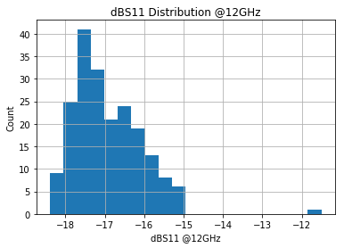
dBS11 Distribution (12GHz)
# Plot dBS11 distribution at 12GHz
df4.dBS11.hist(bins=20)
plt.title('dBS11 Distribution @12GHz')
plt.xlabel('dBS11 @12GHz')
plt.ylabel('Count')
plt.show()
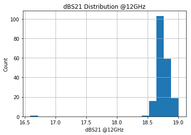
dBS21 Distribution (12GHz)
# Plot dBS21 distribution at 12GHz
df4.dBS21.hist(bins=20)
plt.title('dBS21 Distribution @12GHz')
plt.xlabel('dBS21 @12GHz')
plt.ylabel('Count')
plt.show()
dBS22 Distribution (12GHz)
# Plot dBS22 distribution at 12GHz
df4.dBS22.hist(bins=20)
plt.title('dBS22 Distribution @12GHz')
plt.xlabel('dBS22 @12GHz')
plt.ylabel('Count')
plt.show()
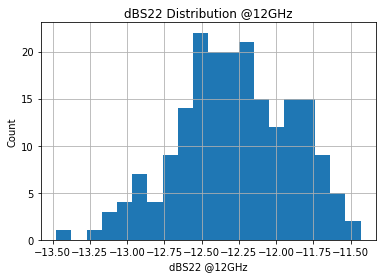
Key Statistics (Freq=12GHz)
df4.describe()
| Freq | dBS11 | dBS21 | dBS22 | |
|---|---|---|---|---|
| count | 199.0 | 199.000000 | 199.000000 | 199.000000 |
| mean | 12.0 | -16.930138 | 18.736482 | -12.274029 |
| std | 0.0 | 0.875090 | 0.176905 | 0.383991 |
| min | 12.0 | -18.389850 | 16.588760 | -13.476270 |
| 25% | 12.0 | -17.531805 | 18.674630 | -12.534845 |
| 50% | 12.0 | -17.092180 | 18.735490 | -12.263640 |
| 75% | 12.0 | -16.350115 | 18.809190 | -11.972370 |
| max | 12.0 | -11.503710 | 19.004470 | -11.433090 |
Extract 14GHz Data
# Extract only the data for Freq = 14
df5 = df.loc[df['Freq'] == 14]
df5.head()
| Freq | dBS11 | dBS21 | dBS22 | |
|---|---|---|---|---|
| 139 | 14.0 | -8.474581 | 18.28153 | -13.63084 |
| 539 | 14.0 | -8.510300 | 18.44825 | -12.29914 |
| 939 | 14.0 | -8.452004 | 18.27976 | -12.87179 |
| 1339 | 14.0 | -10.108590 | 17.75542 | -17.95431 |
| 1739 | 14.0 | -8.592101 | 18.28519 | -12.85863 |
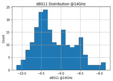
dBS11 Distribution (14GHz)
# Plot dBS11 distribution at 14GHz
df5.dBS11.hist(bins=20)
plt.title('dBS11 Distribution @14GHz')
plt.xlabel('dBS11 @14GHz')
plt.ylabel('Count')
plt.show()
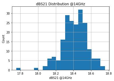
dBS21 Distribution (14GHz)
# Plot dBS21 distribution at 14GHz
df5.dBS21.hist(bins=20)
plt.title('dBS21 Distribution @14GHz')
plt.xlabel('dBS21 @14GHz')
plt.ylabel('Count')
plt.show()
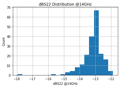
dBS22 Distribution (14GHz)
# Plot dBS22 distribution at 14GHz
df5.dBS22.hist(bins=20)
plt.title('dBS22 Distribution @14GHz')
plt.xlabel('dBS22 @14GHz')
plt.ylabel('Count')
plt.show()
Key Statistics (Freq=14GHz)
df5.describe()
| Freq | dBS11 | dBS21 | dBS22 | |
|---|---|---|---|---|
| count | 199.0 | 199.000000 | 199.000000 | 199.000000 |
| mean | 14.0 | -9.159178 | 18.410712 | -13.184445 |
| std | 0.0 | 0.493677 | 0.144272 | 0.662660 |
| min | 14.0 | -10.144590 | 17.755420 | -17.954310 |
| 25% | 14.0 | -9.534648 | 18.323560 | -13.401830 |
| 50% | 14.0 | -9.264850 | 18.414970 | -13.055440 |
| 75% | 14.0 | -8.805143 | 18.504870 | -12.863730 |
| max | 14.0 | -7.844082 | 18.755250 | -11.882130 |
1805A Data
df = pd.read_csv('docs/F123019_1_B18U01_BST1805A_S_full.csv', delimiter='\;')
df = df.drop(['XAdress', 'YAdress', 'PhS11', 'dBS12', 'PhS12', 'PhS21', 'PhS22', 'Unnamed: 11'], axis=1).dropna()
df.head()
/Users/rakeshbhatia/anaconda/lib/python3.6/site-packages/ipykernel_launcher.py:1: ParserWarning: Falling back to the 'python' engine because the 'c' engine does not support regex separators (separators > 1 char and different from '\s+' are interpreted as regex); you can avoid this warning by specifying engine='python'.
  """Entry point for launching an IPython kernel.
| Freq | dBS11 | dBS21 | dBS22 | |
|---|---|---|---|---|
| 0 | 0.1 | 0.010573 | -76.08674 | -0.013744 |
| 1 | 0.2 | -0.020535 | -69.14332 | -0.098646 |
| 2 | 0.3 | -0.009909 | -63.57820 | -0.185163 |
| 3 | 0.4 | -0.045886 | -58.17558 | -0.292580 |
| 4 | 0.5 | -0.071007 | -50.92647 | -0.416192 |
print(df.dtypes)
Freq     float64
dBS11    float64
dBS21    float64
dBS22    float64
dtype: object
Extract 5GHz Data
# Extract only the data for Freq = 5
df1 = df.loc[df['Freq'] == 5]
df1.head()
| Freq | dBS11 | dBS21 | dBS22 | |
|---|---|---|---|---|
| 49 | 5.0 | -10.42336 | 23.61511 | -11.95370 |
| 449 | 5.0 | -10.40914 | 23.64648 | -12.07714 |
| 849 | 5.0 | -10.18221 | 23.56678 | -11.93713 |
| 1249 | 5.0 | -10.78723 | 23.70150 | -12.13950 |
| 1649 | 5.0 | -10.49322 | 23.59074 | -11.91809 |
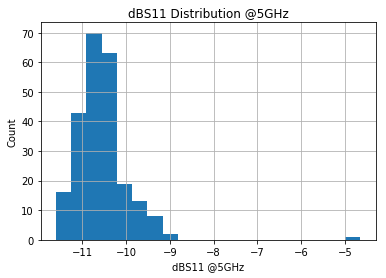
dBS11 Distribution (5GHz)
# Plot dBS11 distribution at 5GHz
df1.dBS11.hist(bins=20)
plt.title('dBS11 Distribution @5GHz')
plt.xlabel('dBS11 @5GHz')
plt.ylabel('Count')
plt.show()
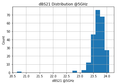
dBS21 Distribution (5GHz)
# Plot dBS21 distribution at 5GHz
df1.dBS21.hist(bins=20)
plt.title('dBS21 Distribution @5GHz')
plt.xlabel('dBS21 @5GHz')
plt.ylabel('Count')
plt.show()
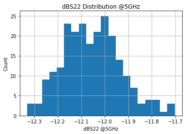
dBS22 Distribution (5GHz)
# Plot dBS22 distribution at 5GHz
df1.dBS22.hist(bins=20)
plt.title('dBS22 Distribution @5GHz')
plt.xlabel('dBS22 @5GHz')
plt.ylabel('Count')
plt.show()
Key Statistics (Freq=5GHz)
df1.describe()
| Freq | dBS11 | dBS21 | dBS22 | |
|---|---|---|---|---|
| count | 235.0 | 235.000000 | 235.000000 | 235.000000 |
| mean | 5.0 | -10.551063 | 23.669021 | -12.054247 |
| std | 0.0 | 0.629894 | 0.277857 | 0.123789 |
| min | 5.0 | -11.601430 | 20.659760 | -12.329980 |
| 25% | 5.0 | -10.904755 | 23.561080 | -12.147175 |
| 50% | 5.0 | -10.595160 | 23.680400 | -12.057860 |
| 75% | 5.0 | -10.372880 | 23.812605 | -11.973135 |
| max | 5.0 | -4.644823 | 24.090790 | -11.702950 |
Extract 7GHz Data
# Extract only the data for Freq = 7
df2 = df.loc[df['Freq'] == 7]
df2.head()
| Freq | dBS11 | dBS21 | dBS22 | |
|---|---|---|---|---|
| 69 | 7.0 | -16.60513 | 22.61904 | -13.15295 |
| 469 | 7.0 | -16.45434 | 22.66301 | -13.46626 |
| 869 | 7.0 | -17.16176 | 22.70254 | -13.10398 |
| 1269 | 7.0 | -16.35508 | 22.68294 | -13.74697 |
| 1669 | 7.0 | -16.81986 | 22.69728 | -13.09944 |
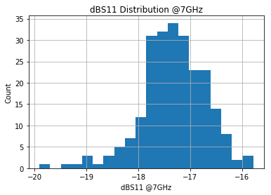
dBS11 Distribution (7GHz)
# Plot dBS11 distribution at 7GHz
df2.dBS11.hist(bins=20)
plt.title('dBS11 Distribution @7GHz')
plt.xlabel('dBS11 @7GHz')
plt.ylabel('Count')
plt.show()
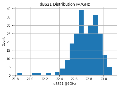
dBS21 Distribution (7GHz)
# Plot dBS21 distribution at 7GHz
df2.dBS21.hist(bins=20)
plt.title('dBS21 Distribution @7GHz')
plt.xlabel('dBS21 @7GHz')
plt.ylabel('Count')
plt.show()
dBS22 Distribution (7GHz)
# Plot dBS22 distribution at 7GHz
df2.dBS22.hist(bins=20)
plt.title('dBS22 Distribution @7GHz')
plt.xlabel('dBS22 @7GHz')
plt.ylabel('Count')
plt.show()
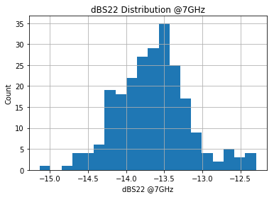
Key Statistics (Freq=7GHz)
df2.describe()
| Freq | dBS11 | dBS21 | dBS22 | |
|---|---|---|---|---|
| count | 235.0 | 235.000000 | 235.000000 | 235.000000 |
| mean | 7.0 | -17.309036 | 22.761961 | -13.644450 |
| std | 0.0 | 0.622652 | 0.178806 | 0.471827 |
| min | 7.0 | -19.906880 | 21.828900 | -15.133200 |
| 25% | 7.0 | -17.653740 | 22.656650 | -13.949530 |
| 50% | 7.0 | -17.303050 | 22.771070 | -13.648070 |
| 75% | 7.0 | -16.892930 | 22.891935 | -13.379725 |
| max | 7.0 | -15.784470 | 23.117140 | -12.296640 |
Extract 11GHz Data
# Extract only the data for Freq = 11
df3 = df.loc[df['Freq'] == 11]
df3.head()
| Freq | dBS11 | dBS21 | dBS22 | |
|---|---|---|---|---|
| 109 | 11.0 | -12.33532 | 22.11853 | -16.49619 |
| 509 | 11.0 | -12.26973 | 22.16444 | -17.07395 |
| 909 | 11.0 | -12.22223 | 22.26095 | -16.53758 |
| 1309 | 11.0 | -12.50065 | 22.19628 | -17.62481 |
| 1709 | 11.0 | -12.31606 | 22.28214 | -16.54425 |
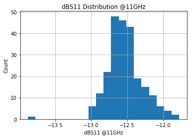
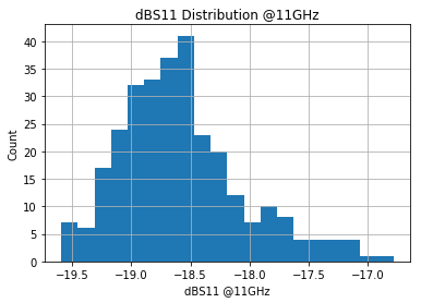
dBS11 Distribution (11GHz)
# Plot dBS11 distribution at 11GHz
df3.dBS11.hist(bins=20)
plt.title('dBS11 Distribution @11GHz')
plt.xlabel('dBS11 @11GHz')
plt.ylabel('Count')
plt.show()
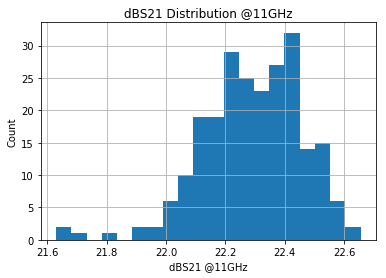
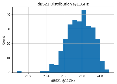
dBS21 Distribution (11GHz)
# Plot dBS21 distribution at 11GHz
df3.dBS21.hist(bins=20)
plt.title('dBS21 Distribution @11GHz')
plt.xlabel('dBS21 @11GHz')
plt.ylabel('Count')
plt.show()
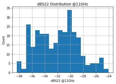
dBS22 Distribution (11GHz)
# Plot dBS22 distribution at 11GHz
df3.dBS22.hist(bins=20)
plt.title('dBS22 Distribution @11GHz')
plt.xlabel('dBS22 @11GHz')
plt.ylabel('Count')
plt.show()
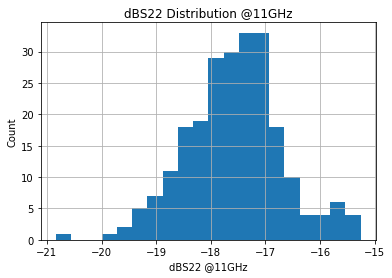
Key Statistics (Freq=11GHz)
df3.describe()
| Freq | dBS11 | dBS21 | dBS22 | |
|---|---|---|---|---|
| count | 235.0 | 235.000000 | 235.000000 | 235.000000 |
| mean | 11.0 | -12.532657 | 22.291133 | -17.561227 |
| std | 0.0 | 0.244757 | 0.170289 | 0.886189 |
| min | 11.0 | -13.881930 | 21.629940 | -20.829990 |
| 25% | 11.0 | -12.660305 | 22.190090 | -18.128210 |
| 50% | 11.0 | -12.552040 | 22.297950 | -17.544260 |
| 75% | 11.0 | -12.412675 | 22.414160 | -17.048630 |
| max | 11.0 | -11.774760 | 22.655760 | -15.258520 |
Extract 18GHz Data
# Extract only the data for Freq = 18
df4 = df.loc[df['Freq'] == 18]
df4.head()
| Freq | dBS11 | dBS21 | dBS22 | |
|---|---|---|---|---|
| 179 | 18.0 | -32.53231 | 20.43977 | -15.92729 |
| 579 | 18.0 | -32.15328 | 20.41885 | -16.01540 |
| 979 | 18.0 | -29.55933 | 20.46294 | -16.28956 |
| 1379 | 18.0 | -33.73080 | 20.32515 | -16.01700 |
| 1779 | 18.0 | -29.81385 | 20.41036 | -16.23384 |
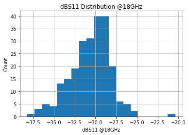
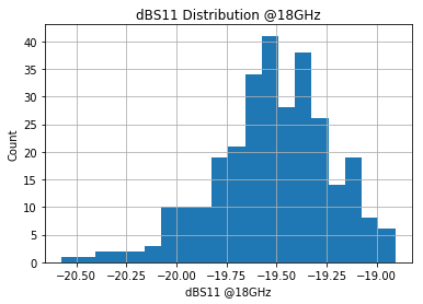
dBS11 Distribution (18GHz)
# Plot dBS11 distribution at 18GHz
df4.dBS11.hist(bins=20)
plt.title('dBS11 Distribution @18GHz')
plt.xlabel('dBS11 @18GHz')
plt.ylabel('Count')
plt.show()
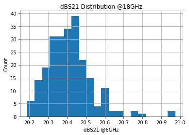
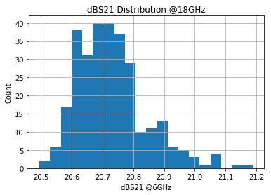
dBS21 Distribution (18GHz)
# Plot dBS21 distribution at 18GHz
df4.dBS21.hist(bins=20)
plt.title('dBS21 Distribution @18GHz')
plt.xlabel('dBS21 @6GHz')
plt.ylabel('Count')
plt.show()
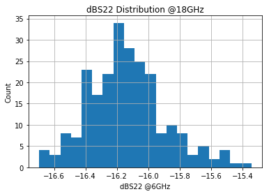
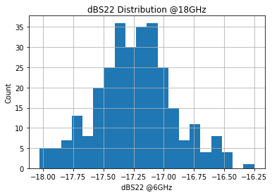
dBS22 Distribution (18GHz)
# Plot dBS22 distribution at 18GHz
df4.dBS22.hist(bins=20)
plt.title('dBS22 Distribution @18GHz')
plt.xlabel('dBS22 @6GHz')
plt.ylabel('Count')
plt.show()
Key Statistics (Freq=18GHz)
df4.describe()
| Freq | dBS11 | dBS21 | dBS22 | |
|---|---|---|---|---|
| count | 235.0 | 235.000000 | 235.000000 | 235.000000 |
| mean | 18.0 | -30.599641 | 20.412133 | -16.137362 |
| std | 0.0 | 2.402802 | 0.118059 | 0.244860 |
| min | 18.0 | -38.203290 | 20.189260 | -16.695290 |
| 25% | 18.0 | -31.991915 | 20.330560 | -16.299205 |
| 50% | 18.0 | -30.235330 | 20.407730 | -16.158040 |
| 75% | 18.0 | -28.964435 | 20.465155 | -16.006095 |
| max | 18.0 | -20.403410 | 20.973560 | -15.344100 |
Extract 20GHz Data
# Extract only the data for Freq = 20
df5 = df.loc[df['Freq'] == 20]
df5.head()
| Freq | dBS11 | dBS21 | dBS22 | |
|---|---|---|---|---|
| 199 | 20.0 | -16.92885 | 18.76583 | -13.90444 |
| 599 | 20.0 | -16.80726 | 18.73182 | -13.84491 |
| 999 | 20.0 | -16.57510 | 18.77656 | -14.09999 |
| 1399 | 20.0 | -16.60360 | 18.64695 | -13.88561 |
| 1799 | 20.0 | -16.17047 | 18.70738 | -13.94949 |
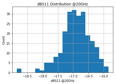
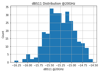
dBS11 Distribution (20GHz)
# Plot dBS11 distribution at 20GHz
df5.dBS11.hist(bins=20)
plt.title('dBS11 Distribution @20GHz')
plt.xlabel('dBS11 @20GHz')
plt.ylabel('Count')
plt.show()
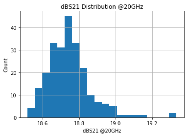
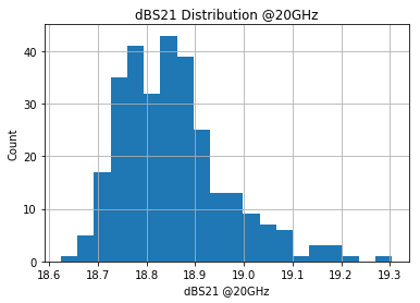
dBS21 Distribution (20GHz)
# Plot dBS21 distribution at 20GHz
df5.dBS21.hist(bins=20)
plt.title('dBS21 Distribution @20GHz')
plt.xlabel('dBS21 @20GHz')
plt.ylabel('Count')
plt.show()
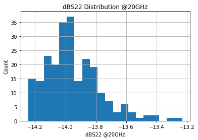
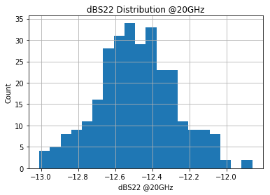
dBS22 Distribution (20GHz)
# Plot dBS22 distribution at 20GHz
df5.dBS22.hist(bins=20)
plt.title('dBS22 Distribution @20GHz')
plt.xlabel('dBS22 @20GHz')
plt.ylabel('Count')
plt.show()
Key Statistics (Freq=20GHz)
df5.describe()
| Freq | dBS11 | dBS21 | dBS22 | |
|---|---|---|---|---|
| count | 235.0 | 235.000000 | 235.000000 | 235.000000 |
| mean | 20.0 | -16.906550 | 18.746694 | -13.947362 |
| std | 0.0 | 0.472049 | 0.119102 | 0.179936 |
| min | 20.0 | -18.841970 | 18.515630 | -14.244200 |
| 25% | 20.0 | -17.172030 | 18.665670 | -14.075910 |
| 50% | 20.0 | -16.889640 | 18.735730 | -13.966830 |
| 75% | 20.0 | -16.603455 | 18.798750 | -13.843645 |
| max | 20.0 | -15.846820 | 19.333830 | -13.231020 |
1805B Data
df = pd.read_csv('docs/F123019_1_B18U01_BST1805B_S_full.csv', delimiter='\;')
df = df.drop(['XAdress', 'YAdress', 'PhS11', 'dBS12', 'PhS12', 'PhS21', 'PhS22', 'Unnamed: 11'], axis=1).dropna()
df.head()
/Users/rakeshbhatia/anaconda/lib/python3.6/site-packages/ipykernel_launcher.py:1: ParserWarning: Falling back to the 'python' engine because the 'c' engine does not support regex separators (separators > 1 char and different from '\s+' are interpreted as regex); you can avoid this warning by specifying engine='python'.
  """Entry point for launching an IPython kernel.
| Freq | dBS11 | dBS21 | dBS22 | |
|---|---|---|---|---|
| 0 | 0.1 | -0.010521 | -62.68544 | 0.001049 |
| 1 | 0.2 | -0.021072 | -70.72228 | -0.084547 |
| 2 | 0.3 | -0.015438 | -64.09773 | -0.185811 |
| 3 | 0.4 | -0.030365 | -57.71990 | -0.295006 |
| 4 | 0.5 | -0.064610 | -50.78907 | -0.420105 |
print(df.dtypes)
Freq     float64
dBS11    float64
dBS21    float64
dBS22    float64
dtype: object
Extract 5GHz Data
# Extract only the data for Freq = 5
df1 = df.loc[df['Freq'] == 5]
df1.head()
| Freq | dBS11 | dBS21 | dBS22 | |
|---|---|---|---|---|
| 49 | 5.0 | -11.07842 | 23.67603 | -11.74675 |
| 449 | 5.0 | -10.92548 | 23.73322 | -11.72783 |
| 849 | 5.0 | -11.16697 | 23.71796 | -11.73677 |
| 1249 | 5.0 | -11.07818 | 23.79352 | -11.70459 |
| 1649 | 5.0 | -11.19607 | 23.74428 | -11.68492 |
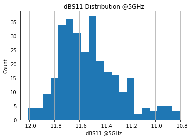
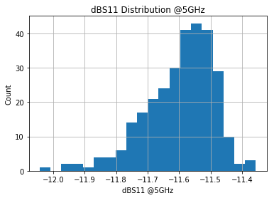
dBS11 Distribution (5GHz)
# Plot dBS11 distribution at 5GHz
df1.dBS11.hist(bins=20)
plt.title('dBS11 Distribution @5GHz')
plt.xlabel('dBS11 @5GHz')
plt.ylabel('Count')
plt.show()
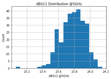
dBS21 Distribution (5GHz)
# Plot dBS21 distribution at 5GHz
df1.dBS21.hist(bins=20)
plt.title('dBS11 Distribution @5GHz')
plt.xlabel('dBS11 @5GHz')
plt.ylabel('Count')
plt.show()
dBS22 Distribution (5GHz)
# Plot dBS22 distribution at 5GHz
df1.dBS22.hist(bins=20)
plt.title('dBS11 Distribution @5GHz')
plt.xlabel('dBS11 @5GHz')
plt.ylabel('Count')
plt.show()
Key Statistics (Freq=5GHz)
df1.describe()
| Freq | dBS11 | dBS21 | dBS22 | |
|---|---|---|---|---|
| count | 295.0 | 295.000000 | 295.000000 | 295.000000 |
| mean | 5.0 | -11.518385 | 23.779997 | -11.597490 |
| std | 0.0 | 0.239181 | 0.151274 | 0.110049 |
| min | 5.0 | -12.009660 | 23.062440 | -12.042890 |
| 25% | 5.0 | -11.695270 | 23.676410 | -11.659265 |
| 50% | 5.0 | -11.550750 | 23.793520 | -11.578470 |
| 75% | 5.0 | -11.383740 | 23.889265 | -11.516745 |
| max | 5.0 | -10.802340 | 24.152850 | -11.356200 |
Extract 7GHz Data
# Extract only the data for Freq = 7
df2 = df.loc[df['Freq'] == 7]
df2.head()
| Freq | dBS11 | dBS21 | dBS22 | |
|---|---|---|---|---|
| 69 | 7.0 | -10.72236 | 22.96420 | -16.36640 |
| 469 | 7.0 | -10.53478 | 23.01464 | -16.51727 |
| 869 | 7.0 | -10.73799 | 23.04493 | -16.29637 |
| 1269 | 7.0 | -10.63710 | 23.07998 | -16.64480 |
| 1669 | 7.0 | -10.70496 | 23.10423 | -16.62696 |
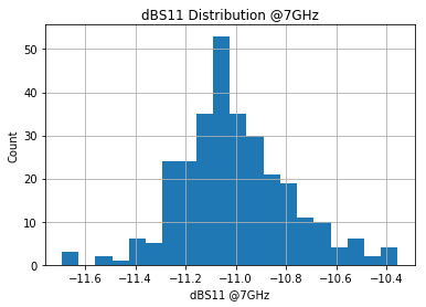
dBS11 Distribution (7GHz)
# Plot dBS11 distribution at 7GHz
df2.dBS11.hist(bins=20)
plt.title('dBS11 Distribution @7GHz')
plt.xlabel('dBS11 @7GHz')
plt.ylabel('Count')
plt.show()
dBS21 Distribution (7GHz)
# Plot dBS21 distribution at 7GHz
df2.dBS21.hist(bins=20)
plt.title('dBS21 Distribution @7GHz')
plt.xlabel('dBS21 @7GHz')
plt.ylabel('Count')
plt.show()
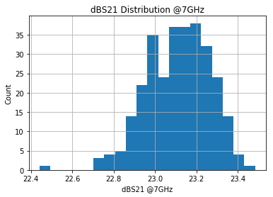
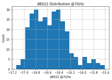
dBS22 Distribution (7GHz)
# Plot dBS22 distribution at 7GHz
df2.dBS22.hist(bins=20)
plt.title('dBS22 Distribution @7GHz')
plt.xlabel('dBS22 @7GHz')
plt.ylabel('Count')
plt.show()
Key Statistics (Freq=7GHz)
df2.describe()
| Freq | dBS11 | dBS21 | dBS22 | |
|---|---|---|---|---|
| count | 295.0 | 295.000000 | 295.000000 | 295.000000 |
| mean | 7.0 | -11.005048 | 23.111815 | -16.542979 |
| std | 0.0 | 0.219449 | 0.152174 | 0.301244 |
| min | 7.0 | -11.692570 | 22.442400 | -17.136980 |
| 25% | 7.0 | -11.138315 | 23.001080 | -16.786150 |
| 50% | 7.0 | -11.032210 | 23.126220 | -16.561240 |
| 75% | 7.0 | -10.883580 | 23.224445 | -16.358780 |
| max | 7.0 | -10.354600 | 23.483890 | -15.609760 |
Extract 11GHz Data
# Extract only the data for Freq = 6
df3 = df.loc[df['Freq'] == 11]
df3.head()
| Freq | dBS11 | dBS21 | dBS22 | |
|---|---|---|---|---|
| 109 | 11.0 | -17.81669 | 23.62515 | -28.44229 |
| 509 | 11.0 | -17.75754 | 23.68512 | -29.67550 |
| 909 | 11.0 | -17.86480 | 23.74452 | -28.42763 |
| 1309 | 11.0 | -18.14783 | 23.73582 | -31.09664 |
| 1709 | 11.0 | -18.10816 | 23.82677 | -31.44076 |
dBS11 Distribution (11GHz)
# Plot dBS11 distribution at 11GHz
df3.dBS11.hist(bins=20)
plt.title('dBS11 Distribution @11GHz')
plt.xlabel('dBS11 @11GHz')
plt.ylabel('Count')
plt.show()
dBS21 Distribution (11GHz)
# Plot dBS21 distribution at 11GHz
df3.dBS21.hist(bins=20)
plt.title('dBS21 Distribution @11GHz')
plt.xlabel('dBS21 @11GHz')
plt.ylabel('Count')
plt.show()
dBS22 Distribution (11GHz)
# Plot dBS22 distribution at 11GHz
df3.dBS22.hist(bins=20)
plt.title('dBS22 Distribution @11GHz')
plt.xlabel('dBS22 @11GHz')
plt.ylabel('Count')
plt.show()
Key Statistics (Freq=11GHz)
df3.describe()
| Freq | dBS11 | dBS21 | dBS22 | |
|---|---|---|---|---|
| count | 295.0 | 295.000000 | 295.000000 | 295.000000 |
| mean | 11.0 | -18.575991 | 23.775733 | -32.004279 |
| std | 0.0 | 0.521307 | 0.144373 | 3.225291 |
| min | 11.0 | -19.592070 | 23.076620 | -38.388420 |
| 25% | 11.0 | -18.943620 | 23.673485 | -34.711460 |
| 50% | 11.0 | -18.629620 | 23.782870 | -31.811210 |
| 75% | 11.0 | -18.322280 | 23.884140 | -29.778345 |
| max | 11.0 | -16.785870 | 24.104350 | -24.049370 |
Extract 18GHz Data
# Extract only the data for Freq = 18
df4 = df.loc[df['Freq'] == 18]
df4.head()
| Freq | dBS11 | dBS21 | dBS22 | |
|---|---|---|---|---|
| 179 | 18.0 | -19.81520 | 20.80170 | -17.44869 |
| 579 | 18.0 | -19.67049 | 20.79345 | -17.27973 |
| 979 | 18.0 | -19.34783 | 20.79048 | -17.65238 |
| 1379 | 18.0 | -19.58426 | 20.73212 | -17.29170 |
| 1779 | 18.0 | -19.29255 | 20.76008 | -17.31918 |
dBS11 Distribution (18GHz)
# Plot dBS11 distribution at 18GHz
df4.dBS11.hist(bins=20)
plt.title('dBS11 Distribution @18GHz')
plt.xlabel('dBS11 @18GHz')
plt.ylabel('Count')
plt.show()
dBS21 Distribution (18GHz)
# Plot dBS21 distribution at 18GHz
df4.dBS21.hist(bins=20)
plt.title('dBS21 Distribution @18GHz')
plt.xlabel('dBS21 @6GHz')
plt.ylabel('Count')
plt.show()
dBS22 Distribution (18GHz)
# Plot dBS22 distribution at 18GHz
df4.dBS22.hist(bins=20)
plt.title('dBS22 Distribution @18GHz')
plt.xlabel('dBS22 @6GHz')
plt.ylabel('Count')
plt.show()
Key Statistics (Freq=18GHz)
df4.describe()
| Freq | dBS11 | dBS21 | dBS22 | |
|---|---|---|---|---|
| count | 295.0 | 295.000000 | 295.000000 | 295.000000 |
| mean | 18.0 | -19.519634 | 20.729409 | -17.237495 |
| std | 0.0 | 0.293053 | 0.114558 | 0.323519 |
| min | 18.0 | -20.573310 | 20.494880 | -18.029100 |
| 25% | 18.0 | -19.680075 | 20.642035 | -17.427095 |
| 50% | 18.0 | -19.503310 | 20.712400 | -17.254220 |
| 75% | 18.0 | -19.326670 | 20.783380 | -17.038840 |
| max | 18.0 | -18.908340 | 21.189640 | -16.251380 |
Extract 20GHz Data
# Extract only the data for Freq = 20
df5 = df.loc[df['Freq'] == 20]
df5.head()
| Freq | dBS11 | dBS21 | dBS22 | |
|---|---|---|---|---|
| 199 | 20.0 | -15.30288 | 18.91892 | -12.61518 |
| 599 | 20.0 | -15.11921 | 18.89940 | -12.51443 |
| 999 | 20.0 | -15.01253 | 18.89355 | -12.63902 |
| 1399 | 20.0 | -15.08008 | 18.85737 | -12.51217 |
| 1799 | 20.0 | -14.96330 | 18.86747 | -12.47076 |
dBS11 Distribution (20GHz)
# Plot dBS11 distribution at 20GHz
df5.dBS11.hist(bins=20)
plt.title('dBS11 Distribution @20GHz')
plt.xlabel('dBS11 @20GHz')
plt.ylabel('Count')
plt.show()
dBS21 Distribution (20GHz)
# Plot dBS21 distribution at 20GHz
df5.dBS21.hist(bins=20)
plt.title('dBS21 Distribution @20GHz')
plt.xlabel('dBS21 @20GHz')
plt.ylabel('Count')
plt.show()
dBS22 Distribution (20GHz)
# Plot dBS22 distribution at 20GHz
df5.dBS22.hist(bins=20)
plt.title('dBS22 Distribution @20GHz')
plt.xlabel('dBS22 @20GHz')
plt.ylabel('Count')
plt.show()
Key Statistics (Freq=20GHz)
df5.describe()
| Freq | dBS11 | dBS21 | dBS22 | |
|---|---|---|---|---|
| count | 295.0 | 295.000000 | 295.000000 | 295.000000 |
| mean | 20.0 | -15.250557 | 18.854922 | -12.482376 |
| std | 0.0 | 0.315852 | 0.109637 | 0.212733 |
| min | 20.0 | -16.296750 | 18.624680 | -13.008910 |
| 25% | 20.0 | -15.460500 | 18.777085 | -12.621625 |
| 50% | 20.0 | -15.261350 | 18.839660 | -12.489760 |
| 75% | 20.0 | -15.025800 | 18.908925 | -12.347590 |
| max | 20.0 | -14.518400 | 19.304680 | -11.860950 |